1.8.5: Algebra of Vectors

Learning Objectives

• Apply analytical methods of vector algebra to find resultant vectors and to solve vector equations for unknown vectors.
• Interpret physical situations in terms of vector expressions.

Algebra of Vectors

Vectors can be added together and multiplied by scalars. Vector addition is associative and commutative, and vector multiplication by a sum of scalars is distributive. Also, scalar multiplication by a sum of vectors is distributive:

\[\alpha(\vec{A} + \vec{B}) = \alpha \vec{A} + \alpha\vec{B} \ldotp \label{a_vec_01}\]

In this equation, \(\alpha\) is any number (a scalar). For example, a vector antiparallel to vector \(\vec{A}\) = A_x \(\hat{i}\) + A_y \(\hat{j}\) + A_z \(\hat{k}\) can be expressed simply by multiplying \(\vec{A}\) by the scalar \(\alpha\) = −1:\[- \vec{A} = - A_{x} \hat{i} - A_{y} \hat{j} - A_{z} \hat{k} \ldotp \label{a_vec_02}\]

The generalization of the number zero to vector algebra is called the null vector, denoted by \(\vec{0}\). All components of the null vector are zero, \(\vec{0}\) = 0 \(\hat{i}\)+ 0 \(\hat{j}\) + 0 \(\hat{k}\), so the null vector has no length and no direction.

Two vectors \(\vec{A}\) and \(\vec{B}\) are equal vectors if and only if their difference is the null vector: \(\vec{0}\) = \(\vec{A}\) − \(\vec{B}\) = (A_x \(\hat{i}\) + A_y \(\hat{j}\) + A_z \(\hat{k}\)) − (B_x \(\hat{i}\) + B_y \(\hat{j}\) + B_z \(\hat{k}\)) = (A_x − B_x) \(\hat{i}\) + (A_y − B_y) \(\hat{j}\) + (A_z − B_z) \(\hat{k}\). This vector equation means we must have simultaneously A_x − B_x = 0, A_y − B_y = 0, and A_z − B_z = 0. Hence, we can write \(\vec{A} = \vec{B}\) if and only if the corresponding components of vectors \(\vec{A}\) and \(\vec{B}\) are equal:

\[ \vec{A} = \vec{B} \Leftrightarrow \begin{cases} A_{x} = B_{x} \\ A_{y} = B_{y} \\ A_{z} = B_{z} \end{cases} \ldotp \label{a_vec_03}\]

Two vectors are equal when their corresponding scalar components are equal. Resolving vectors into their scalar components (i.e., finding their scalar components) and expressing them analytically in vector component form allows us to use vector algebra to find sums or differences of many vectors analytically (i.e., without using graphical methods). For example, to find the resultant of two vectors \(\vec{A}\) and \(\vec{B}\), we simply add them component by component, as follows:

\[\vec{R} = \vec{A} + \vec{B} = (A_{x}\; \hat{i} + A_{y}\; \hat{j} + A_{z}\; \hat{k}) + (B_{x}\; \hat{i} + B_{y}\; \hat{j} + B_{z}\; \hat{k}) = (A_{x} + B_{x})\; \hat{i} + (A_{y} + B_{y})\; \hat{j} + (A_{z} + B_{z})\; \hat{k} \ldotp \label{a_vec_04}\]

In this way, using Equation \ref{a_vec_04}, scalar components of the resultant vector \(\vec{R}\) = R_x \(\hat{i}\) + R_y \(\hat{j}\) + R_z \(\hat{k}\) are the sums of corresponding scalar components of vectors \(\vec{A}\) and \(\vec{B}\):

\[ \begin{cases} R_{x} = A_{x} + B_{x}, \\ R_{y} = A_{y} + B_{y}, \\ R_{z} = A_{z} + B_{z} \end{cases} \ldotp\]

Analytical methods can be used to find components of a resultant of many vectors. For example, if we are to sum up N vectors \(\vec{F}_{1}\), \(\vec{F}_{2}\), \(\vec{F}_{3}\), … , \(\vec{F}_{N}\), where each vector is \(\vec{F}_{k}\) = F_kx \(\hat{i}\) + F_ky \(\hat{j}\) + F_kz \(\hat{k}\), the resultant vector \(\vec{F}_{R}\) is

\[ \vec{F}_{R} = \vec{F}_{1} + \vec{F}_{2} + \vec{F}_{3} + \ldots + \vec{F}_{N} = \sum_{k = 1}^{N} \vec{F}_{k} = \sum_{k = 1}^{N} \big(F_{kx} \hat{i} + F_{ky} \hat{j} + F_{kz} \hat{k}\big) = \bigg(\sum_{k = 1}^{N} F_{kx}\bigg) \hat{i} + \bigg(\sum_{k = 1}^{N} F_{ky}\bigg) \hat{j} + \bigg(\sum_{k = 1}^{N} F_{kz}\bigg) \hat{k} \ldotp\label{a_vec_05}\]

Therefore, scalar components of the resultant vector are

\[ \begin{cases} F_{Rx} = \sum_{k = 1}^{N} F_{kx} = F_{1x} + F_{2x} + \ldots + F_{Nx} \\ F_{Ry} = \sum_{k = 1}^{N} F_{ky} = F_{1y} + F_{2y} + \ldots + F_{Ny} \\ F_{Rz} = \sum_{k = 1}^{N} F_{kz} = F_{1z} + F_{2z} + \ldots + F_{Nz} \ldotp \end{cases} \label{a_vec_06}\]

Having found the scalar components, we can write the resultant in vector component form:

\[\vec{F}_{R} = F_{Rx}\; \hat{i} + F_{Ry}\; \hat{j} + F_{Rz}\; \hat{k} \ldotp\label{a_vec_07}\]

Analytical methods for finding the resultant and, in general, for solving vector equations are very important in physics because many physical quantities are vectors. For example, we use this method in kinematics to find resultant displacement vectors and resultant velocity vectors, in mechanics to find resultant force vectors and the resultants of many derived vector quantities, and in electricity and magnetism to find resultant electric or magnetic vector fields.

In many physical situations, we often need to know the direction of a vector. For example, we may want to know the direction of a magnetic field vector at some point or the direction of motion of an object. We have already said direction is given by a unit vector, which is a dimensionless entity—that is, it has no physical units associated with it. When the vector in question lies along one of the axes in a Cartesian system of coordinates, the answer is simple, because then its unit vector of direction is either parallel or antiparallel to the direction of the unit vector of an axis. For example, the direction of vector \(\vec{d}\) = −5 m \(\hat{i}\) is unit vector \(\hat{d}\) = − \(\hat{i}\). The general rule of finding the unit vector \(\hat{v}\) of direction for any vector \(\vec{v}\) is to divide it by its magnitude \(|\vec{v}|=v\) :

\[\hat{v} = \frac{\vec{v}}{|\vec{v}|} = \frac{\vec{v}}{v} \ldotp \label{a_vec_08}\]

We see from this expression that the unit vector of direction is indeed dimensionless because the numerator and the denominator in Equation \ref{a_vec_08} have the same physical unit. In this way, Equation \ref{a_vec_08} allows us to express the unit vector of direction in terms of unit vectors of the axes.

Examples

Example \(\PageIndex{1}\): Direction of Motion

In a Cartesian coordinate system where \(\hat{i}\) denotes geographic east, \(\hat{j}\) denotes geographic north, and \(\hat{k}\) denotes altitude above sea level, a military convoy advances its position through unknown territory with velocity \(\vec{v}\) = (4.0 \(\hat{i}\) + 3.0 \(\hat{j}\) + 0.1 \(\hat{k}\)) km/h. If the convoy had to retreat, in what geographic direction would it be moving?

Solution

The velocity vector has the third component \(\vec{v}_{z}\) = (+ 0.1 km/h) \(\hat{k}\), which says the convoy is climbing at a rate of 100 m/h through mountainous terrain. At the same time, its velocity is 4.0 km/h to the east and 3.0 km/h to the north, so it moves on the ground in direction tan⁻¹ (3 /4) ≈ 37° north of east. If the convoy had to retreat, its new velocity vector \(\vec{u}\) would have to be antiparallel to \(\vec{v}\) and be in the form \(\vec{u} = - \alpha \vec{v}\), where \(\alpha\) is a positive number. Thus, the velocity of the retreat would be \(\vec{u}\) = \(\alpha\)(−4.0 \(\hat{i}\) − 3.0 \(\hat{j}\) − 0.1 \(\hat{k}\)) km/h. The negative sign of the third component indicates the convoy would be descending. The direction angle of the retreat velocity is tan⁻¹ (−3 \(\alpha\) − 4 \(\alpha\)) ≈ 37° south of west. Therefore, the convoy would be moving on the ground in direction 37° south of west while descending on its way back.

Example \(\PageIndex{2}\): Analytical Computation of a Resultant

Three displacement vectors \(\vec{A}\), \(\vec{B}\), and \(\vec{C}\) in a plane are specified by their magnitudes A = 10.0, B = 7.0, and C = 8.0, respectively, and by their respective direction angles with the horizontal direction \(\alpha\) = 35°, \(\beta\) = −110°, and \(\gamma\) = 30°. The physical units of the magnitudes are centimeters. Resolve the vectors to their scalar components and find the following vector sums:

1. \(\vec{R}\) = \(\vec{A}\) + \(\vec{B}\) + \(\vec{C}\),
2. \(\vec{D}\) = \(\vec{A}\) − \(\vec{B}\), and
3. \(\vec{S}\) = \(\vec{A}\) − 3 \(\vec{B}\) + \(\vec{C}\).

Strategy

First, we find the scalar components of each vector and then we express each vector in its vector component form given by \(\overrightarrow{\mathbf{A}}=A_{x} \hat{\mathbf{i}}+A_{y} \hat{\mathbf{j}}\). Then, we use analytical methods of vector algebra to find the resultants.

Solution

We resolve the given vectors to their scalar components:

\[ \begin{cases} A_{x} = A \cos \alpha = (10.0\; cm) \cos {35^{o}} = 8.19\; cm \\ A_{y} = A \sin \alpha = (10.0\; cm) \sin{35^{o}} = 5.73\; cm \end{cases}\]

\[ \begin{cases} B_{x} = B \cos \beta = (7.0\; cm) \cos (-110^{o}) = -2.39\; cm \\ B_{y} = B \sin \beta= (7.0\; cm) \sin (-110^{o}) = -6.58\; cm \end{cases}\]

\[ \begin{cases} C_{x} = C \cos \gamma= (8.0\; cm) \cos (30^{o}) = 6.93\; cm \\ C_{y} = C \sin \gamma= (8.0\; cm) \sin(30^{o}) = 4.00\; cm \end{cases}\]

For (a) we may substitute directly into Equation \ref{a_vec_06} to find the scalar components of the resultant:

\[ \begin{cases} R_{x} = A_{x} + B_{x} + C_{x} = 8.19\; cm - 2.39\; cm + 6.93\; cm = 12.73\; cm \\ R_{y} = A_{y} + B_{y} + C_{y} = 5.73\; cm - 6.58\; cm + 4.00\; cm = 3.15\; cm \end{cases}\]

Therefore, the resultant vector is \(\vec{R} = R_{x} \hat{i} + R_{y} \hat{j} = (12.7 \hat{i} + 3.1 \hat{j})\)cm. 

For (b), we may want to write the vector difference as

\[\vec{D} = \vec{A} - \vec{B} = (A_{x} \hat{i} + A_{y} \hat{j}) - (B_{x} \hat{i} + B_{y} \hat{j}) = (A_{x} - B_{x}) \hat{i} + (A_{y} - B_{y}) \hat{j} \ldotp\]

Hence the difference vector is \(\vec{D} = D_{x} \hat{i} + D_{y} \hat{j} = (10.6 \hat{i} + 12.3 \hat{j})\)cm.

For (c), we can write vector \(\vec{S}\) in the following explicit form:

\[ \vec{S} = \vec{A} - 3 \vec{B} + \vec{C} = (A_{x} \hat{i} + A_{y} \hat{j}) - 3(B_{x} \hat{i} + B_{y} \hat{j}) + (C_{x} \hat{i} + C_{y} \hat{j}) = (A_{x} - 3 B_{x} + C_{x}) \hat{i} + (A_{y} - 3 B_{y} + C_{y}) \hat{j} \ldotp\]

Then, the scalar components of \(\vec{S}\) are

\[ \begin{cases} S_{x} = A_{x} - 3B_{x} + C_{x} = 8.19\; cm - 3(-2.39\; cm) + 6.93\; cm = 22.29\; cm \\ S_{y} = A_{y} - 3B_{y} + C_{y} = 5.73\; cm -3(-6.58\; cm) + 4.00\; cm = 29.47\; cm \end{cases}\]

The vector is \(\vec{S} = S_{x} \hat{i} + S_{y} \hat{j} = (22.3 \hat{i} + 29.5 \hat{j})\)cm.

Significance

Having found the vector components, we can illustrate the vectors by graphing or we can compute magnitudes and direction angles, as shown in Figure \(\PageIndex{1}\). Results for the magnitudes in (b) and (c) can be compared with results for the same problems obtained with the graphical method.

Figure \(\PageIndex{1}\): Graphical illustration of the solutions obtained analytically.

Example \(\PageIndex{3}\): The Tug-of-War Game

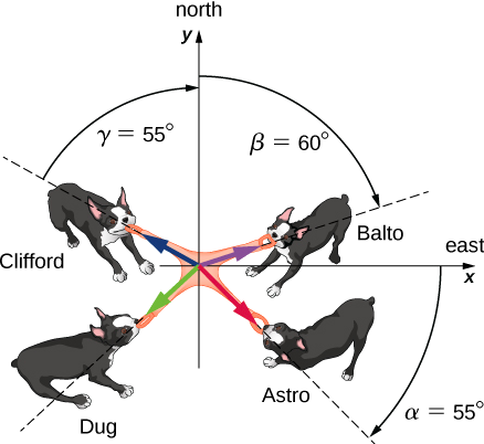
Four dogs named Astro, Balto, Clifford, and Dug play a tug-of-war game with a toy (Figure \(\PageIndex{2}\)). Astro pulls on the toy in direction \(\alpha\) = 55° south of east, Balto pulls in direction \(\beta\) = 60° east of north, and Clifford pulls in direction \(\gamma\) = 55° west of north. Astro pulls strongly with 160.0 units of force (N), which we abbreviate as A = 160.0 N. Balto pulls even stronger than Astro with a force of magnitude B = 200.0 N, and Clifford pulls with a force of magnitude C = 140.0 N. When Dug pulls on the toy in such a way that his force balances out the resultant of the other three forces, the toy does not move in any direction. With how big a force and in what direction must Dug pull on the toy for this to happen?

Figure \(\PageIndex{2}\): Four dogs play a tug-of-war game with a toy.

 

Strategy

We assume that east is the direction of the positive x-axis and north is the direction of the positive y-axis. As in Example \(\PageIndex{1}\), we have to resolve the three given forces — \(\vec{A}\) (the pull from Astro), \(\vec{B}\) (the pull from Balto), and \(\vec{C}\) (the pull from Clifford)—into their scalar components and then find the scalar components of the resultant vector \(\vec{R}\) = \(\vec{A}\) + \(\vec{B}\) + \(\vec{C}\). When the pulling force \(\vec{D}\) from Dug balances out this resultant, the sum of \(\vec{D}\) and \(\vec{R}\) must give the null vector \(\vec{D}\) + \(\vec{R}\) = \(\vec{0}\). This means that \(\vec{D}\) = \(- \vec{R}\) so the pull from Dug must be antiparallel to \(\vec{R}\).

Solution

The direction angles are \(\theta_{A}\) = \(− \alpha\) = −55°, \(\theta_{B}\) = 90° − \(\beta\) = 30°, and \(\theta_{C}\) = 90° + \(\gamma\) = 145°, and substituting them into \ref{a_vec_06} gives the scalar components of the three given forces:

\[ \begin{cases} A_{x} = A \cos \theta_{A} = (160.0\; N) \cos (-55^{o}) = + 91.8\; N \\ A_{y} = A \sin \theta_{A} = (160.0\; N) \sin (-55^{o}) = -131.1\; N \end{cases}\]

\[ \begin{cases} B_{x} = B \cos \theta_{B} = (200.0\; N) \cos 30^{o} = + 173.2\; N \\ B_{y} = B \sin \theta_{B} = (200.0\; N) \sin 30^{o} = + 100.0\; N \end{cases}\]

\[ \begin{cases} C_{x} = C \cos \theta_{C} = (140.0\; N) \cos 145^{o} = -114.7\; N \\ C_{y} = C \sin \theta_{C} = (140.0\; N) \sin 145^{o} = + 80.3\; N \end{cases}\]

Now we compute scalar components of the resultant vector \(\vec{R} = \vec{A} + \vec{B} + \vec{C}\):

\[ \begin{cases} R_{x} = A_{x} + B_{x} + C_{x} = + 91.8\; N+ 173.2\; N- 114.7\; N = +150.3 \; N\\ R_{y} = A_{y} + B_{y} + C_{y} = -131.1\; N + 100.0\; N + 80.3\; N= +49.2\; N\end{cases}\]

The antiparallel vector to the resultant \(\vec{R}\) is

\[\vec{D} = -\vec{R} = -R_{x} \hat{i} - R_{y} \hat{j} = (-150.3 \hat{i} - 49.2 \hat{j}) N \ldotp\]

The magnitude of Dug's pulling force is

\[D = \sqrt{D_{x}^{2} + D_{y}^{2}} = \sqrt{(-150.3)^{2} + (-49.2)^{2}} N = 158.1\; N \ldotp\]

The direction of Dug's pulling force is

\[\theta = \tan^{-1} \left(\dfrac{D_{y}}{D_{x}}\right) = \tan^{-1} \left(\dfrac{-49.2\; N}{-150.3\; N}\right) = \tan^{-1} \left(\dfrac{49.2}{150.3}\right) = 18.1^{o}\ldotp\]

Dug pulls in the direction 18.1° south of west because both components are negative, which means the pull vector lies in the third quadrant.

Example \(\PageIndex{4}\): Vector Algebra

Find the magnitude of the vector \(\vec{C}\) that satisfies the equation 2 \(\vec{A}\) − 6 \(\vec{B}\) + 3 \(\vec{C}\) = 2 \(\hat{j}\), \(\vec{A}\) = \(\hat{i}\) − 2\(\hat{k}\) and \(\vec{B}\) = − \(\hat{j}\) + \(\frac{1}{2} \hat{k}\).

Strategy

We first solve the given equation for the unknown vector \(\vec{C}\). Then we substitute \(\vec{A}\) and \(\vec{B}\); group the terms along each of the three directions \(\hat{i}\), \(\hat{j}\), and \(\hat{k}\); and identify the scalar components C_x, C_y, and C_z. Finally, we substitute into \ref{a_vec_06} to find magnitude C.

Solution

\[\begin{split} 2 \vec{A} - 6 \vec{B} +& 3 \vec{C} = 2 \hat{j}\\ & 3 \vec{C} = 2 \hat{j} - 2 \vec{A} + 6 \vec{B} \\ &\vec{C} = \frac{2}{3} \hat{j} - \frac{2}{3} \vec{A} + 2 \vec{B}\\ & \quad = \frac{2}{3} \hat{j} - \frac{2}{3} (\hat{i} - 2\hat{k}) + 2 \big(- \hat{j} + \frac{1}{2} \hat{k}\big)\\ & \quad = \frac{2}{3} \hat{j} - \frac{2}{3} \hat{i} + \frac{4}{3} \hat{k} - 2 \hat{j} + \hat{k}\\ & \quad = -\frac{2}{3} \hat{i} + \big(\frac{2}{3} - 2 \big)\hat{j} + \big(\frac{4}{3}\ + 1 \big)\hat{k}\\ & \quad = -\frac{2}{3} \hat{i} - \frac{4}{3} \hat{j} + \frac{7}{3} \hat{k} \end{split}\]

The components are C_x = \(-\frac{2}{3}\), C_y = \(-\frac{4}{3}\), and C_z = \(\frac{7}{3}\), and substituting into \ref{a_vec_06} gives

\[C = \sqrt{C_{x}^{2} + C_{y}^{2} + C_{z}^{2}} = \sqrt{\left(-\dfrac{2}{3}\right)^{2} + \left(-\dfrac{4}{3}\right)^{2} + \left(\dfrac{7}{3}\right)^{2}} = \sqrt{\frac{23}{3}} \ldotp\]

Example \(\PageIndex{5}\): Displacement of a Skier

Starting at a ski lodge, a cross-country skier goes 5.0 km north, then 3.0 km west, and finally 4.0 km southwest before taking a rest. Find his total displacement vector relative to the lodge when he is at the rest point. How far and in what direction must he ski from the rest point to return directly to the lodge?

Strategy

We assume a rectangular coordinate system with the origin at the ski lodge and with the unit vector \(\hat{i}\) pointing east and the unit vector \(\hat{j}\) pointing north. There are three displacements: \(\vec{D}_{1}\), \(\vec{D}_{2}\), and \(\vec{D}_{3}\). We identify their magnitudes as D₁ = 5.0 km , D₂ = 3.0 km , and D₃ = 4.0 km . We identify their directions are the angles \(\theta_{1}\) = 90°, \(\theta_{2}\) = 180°, and \(\theta_{3}\) = 180° + 45° = 225°. We resolve each displacement vector to its scalar components and substitute the components into \ref{a_vec_06} to obtain the scalar components of the resultant displacement \(\vec{D}\) from the lodge to the rest point. On the way back from the rest point to the lodge, the displacement is \(\vec{B}\) = − \(\vec{D}\). Finally, we find the magnitude and direction of \(\vec{B}\).

Solution

Scalar components of the displacement vectors are

\[ \begin{cases} D_{1x} = D_{1} \cos \theta_{1} = (5.0\; km) \cos 90^{o} = 0 \\ D_{1y} = D_{1} \sin \theta_{1} = (5.0\; km) \sin 90^{o} = 5.0\; km \end{cases}\]

\[ \begin{cases} D_{2x} = D_{2} \cos \theta_{2} = (3.0\; km) \cos 180^{o} = -3.0 \;km\\ D_{2y} = D_{2} \sin \theta_{2} = (3.0\; km) \sin 180^{o} = 0 \end{cases}\]

\[ \begin{cases} D_{3x} = D_{3} \cos \theta_{3} = (4.0\; km) \cos 225^{o} = -2.8\; km \\ D_{3y} = D_{3} \sin \theta_{3} = (4.0\; km) \sin 225^{o} = -2.8\; km \end{cases}\]

Scalar components of the net displacement vector are

\[ \begin{cases} D_{x} = D_{1x} + D_{2x} + D_{3x} = (0 - 3.0 - 2.8)km = -5.8\; km \\ D_{y} = D_{1y} + D_{2y} + D_{3y} = (5.0 + 0 - 2.8)km = + 2.2\; km \end{cases}\]

Hence, the skier’s net displacement vector is \(\vec{D}\) = D_x \(\hat{i}\) + D_y \(\hat{j}\) = (−5.8 \(\hat{i}\) + 2.2 \(\hat{j}\))km . On the way back to the lodge, his displacement is \(\vec{B}\) = − \(\vec{D}\) = −(−5.8 \(\hat{i}\)+ 2.2 \(\hat{j}\))km = (5.8 \(\hat{i}\) − 2.2 \(\hat{j}\))km. Its magnitude is B = \(\sqrt{B_{x}^{2} + B_{y}^{2}}\) = \(\sqrt{(5.8)^{2} + (−2.2)^{2}}\) km = 6.2 km and its direction angle is \(\theta\)= tan⁻¹\(\left(\dfrac{−2.2}{5.8}\right)\) = −20.8°. Therefore, to return to the lodge, he must go 6.2 km in a direction about 21° south of east.

Significance

Notice that no figure is needed to solve this problem by the analytical method. Figures are required when using a graphical method; however, we can check if our solution makes sense by sketching it, which is a useful final step in solving any vector problem.

Example \(\PageIndex{6}\): Displacement of a Jogger

A jogger runs up a flight of 200 identical steps to the top of a hill and then runs along the top of the hill 50.0 m before he stops at a drinking fountain (Figure \(\PageIndex{3}\)). His displacement vector from point A at the bottom of the steps to point B at the fountain is \(\vec{D}_{AB}\) = (−90.0 \(\hat{i}\) + 30.0 \(\hat{j}\))m. What is the height and width of each step in the flight? What is the actual distance the jogger covers? If he makes a loop and returns to point A, what is his net displacement vector?

Figure \(\PageIndex{3}\): A jogger runs up a flight of steps.

 

Strategy

The displacement vector \(\vec{D}_{AB}\) is the vector sum of the jogger’s displacement vector \(\vec{D}_{AT}\) along the stairs (from point A at the bottom of the stairs to point T at the top of the stairs) and his displacement vector \(\vec{D}_{RB}\) on the top of the hill (from point T at the top of the stairs to the fountain at point B). We must find the horizontal and the vertical components of \(\vec{D}_{TB}\). If each step has width w and height h, the horizontal component of \(\vec{D}_{TB}\) must have a length of 200w and the vertical component must have a length of 200h. The actual distance the jogger covers is the sum of the distance he runs up the stairs and the distance of 50.0 m that he runs along the top of the hill.

Solution

In the coordinate system indicated in Figure \(\PageIndex{3}\), the jogger’s displacement vector on the top of the hill is \(\vec{D}_{RB}\) = (−50.0 m) \(\hat{i}\). His net displacement vector is

\[\vec{D}_{AB} = \vec{D}_{AT} + \vec{D}_{TB} \ldotp \nonumber\]

Therefore, his displacement vector \(\vec{D}_{TB}\) along the stairs is

\[\begin{split} \vec{D}_{AT}& = \vec{D}_{AB} - \vec{D}_{TB} = (-90.0 \hat{i} + 30.0 \hat{j})m - (-50.0 m)\hat{i}) = [(-90.0 50.0) hat{i} + 30.0 \hat{j})]m \\ & = (-40.0 \hat{i} + 30.0 \hat{j})m \ldotp \end{split}\]

Its scalar components are D_ATx = −40.0 m and D_ATy = 30.0 m. Therefore, we must have

\[200 w=|-40.0| \mathrm{m} \text { and } 200 h=30.0 \: \mathrm{m} \ldotp \nonumber\]

Hence, the step width is w = \(\frac{40.0\; m}{200}\) = 0.2 m = 20 cm, and the step height is w = \(\frac{30.0\; m}{200}\) = 0.15 m = 15 cm. The distance that the jogger covers along the stairs is

\[\vec{D}_{AT} = \sqrt{\vec{D}_{ATx}^{2} + \vec{D}_{ATy}^{2}} = \sqrt{(-40.0)^{2} + (30.0)^{2}}m = 50.0\; m \ldotp \nonumber\]

Thus, the actual distance he runs is D_AT + D_TB = 50.0 m + 50.0 m = 100.0 m. When he makes a loop and comes back from the fountain to his initial position at point A, the total distance he covers is twice this distance,or 200.0 m. However, his net displacement vector is zero, because when his final position is the same as his initial position, the scalar components of his net displacement vector are zero (\ref{a_vec_06}).

Example \(\PageIndex{7}\): The Unit Vector of Direction

If the velocity vector of the military convoy is \(\vec{v}\) = (4.000 \(\hat{i}\) + 3.000 \(\hat{j}\) + 0.100 \(\hat{k}\))km/h, what is the unit vector of its direction of motion.

Strategy

The unit vector of the convoy’s direction of motion is the unit vector \(\hat{v}\) that is parallel to the velocity vector. The unit vector is obtained by dividing a vector by its magnitude, in accordance with Equation \ref{2.26}.

Solution

The magnitude of the vector \(\vec{v}\) is

\[v = \sqrt{v_{x}^{2} + v_{y}^{2} + v_{z}^{2}} = \sqrt{4.000^{2} + 3.000^{2} + 0.100^{2}}km/h = 5.001\; km/h \ldotp \nonumber\]

To obtain the unit vector \(\hat{v}\), divide \(\vec{v}\) by its magnitude:

\[\begin{split} \hat{v}& = \frac{\vec{v}}{v} = \frac{(4.000 \hat{i} + 3.00 \hat{j} + 0.100 \hat{k})km/h}{5.001\; km/h} \\ & = \frac{(4.000 \hat{i} + 3.000 \hat{j} + 0.1100 \hat{k})}{5.001} \\ & = \frac{4.000}{5.001} \hat{i} + \frac{3.000}{5.001} \hat{j} + \frac{0.100}{5.001} \hat{k} \\ & = (79.98 \hat{i} + 59.99 \hat{j} + 2.00 \hat{k}) \times 10^{-2} \ldotp \end{split}\]

Significance

Note that when using the analytical method with a calculator, it is advisable to carry out your calculations to at least three decimal places and then round off the final answer to the required number of significant figures, which is the way we performed calculations in this example. If you round off your partial answer too early, you risk your final answer having a huge numerical error, and it may be far off from the exact answer or from a value measured in an experiment.

Contributors

• Samuel J. Ling (Truman State University), Jeff Sanny (Loyola Marymount University), and Bill Moebs with many contributing authors. This work is licensed by OpenStax University Physics under a Creative Commons Attribution License (by 4.0).