6.2: Angular Momentum and Torque

Last updated
Save as PDF

Page ID: 63159

\( \newcommand{\vecs}[1]{\overset { \scriptstyle \rightharpoonup} {\mathbf{#1}} } \) \( \newcommand{\vecd}[1]{\overset{-\!-\!\rightharpoonup}{\vphantom{a}\smash {#1}}} \)\(\newcommand{\id}{\mathrm{id}}\) \( \newcommand{\Span}{\mathrm{span}}\) \( \newcommand{\kernel}{\mathrm{null}\,}\) \( \newcommand{\range}{\mathrm{range}\,}\) \( \newcommand{\RealPart}{\mathrm{Re}}\) \( \newcommand{\ImaginaryPart}{\mathrm{Im}}\) \( \newcommand{\Argument}{\mathrm{Arg}}\) \( \newcommand{\norm}[1]{\| #1 \|}\) \( \newcommand{\inner}[2]{\langle #1, #2 \rangle}\) \( \newcommand{\Span}{\mathrm{span}}\) \(\newcommand{\id}{\mathrm{id}}\) \( \newcommand{\Span}{\mathrm{span}}\) \( \newcommand{\kernel}{\mathrm{null}\,}\) \( \newcommand{\range}{\mathrm{range}\,}\) \( \newcommand{\RealPart}{\mathrm{Re}}\) \( \newcommand{\ImaginaryPart}{\mathrm{Im}}\) \( \newcommand{\Argument}{\mathrm{Arg}}\) \( \newcommand{\norm}[1]{\| #1 \|}\) \( \newcommand{\inner}[2]{\langle #1, #2 \rangle}\) \( \newcommand{\Span}{\mathrm{span}}\)\(\newcommand{\AA}{\unicode[.8,0]{x212B}}\)

So far, we have seen that angular momentum is conserved in the same way that linear momentum is conserved. Specifically, in a system which can be modeled as isolated, angular momentum is conserved,

\[\Delta \vec{L}=0,\]

in the same way that linear momentum was, \(\Delta \vec{p}=0\). There is another similarity between these two cases - when the system was not isolated, we could model the interactions between the system and the environment by a force \(\vec{F}\) acting over a time period \(\Delta t\), so that

\[\vec{F}=\frac{\Delta \vec{p}}{\Delta t}\rightarrow \Delta \vec{p}=\vec{F}\Delta t.\]

In other words, if the system is not isolated we can still work with \(\Delta \vec{p}\), we just have to set it equal to the (net) force times the time interval, rather than simply zero.

There is a similar expression for angular momentum - when a system experiences a change in angular momentum \(\Delta \vec{L}\) over a time period \(\Delta t\) due to an external interaction of some kind, we can model that interaction as delivering a torque \(\vec{\tau}\) to the system, defined as

\[\vec{\tau}=\frac{\Delta \vec{L}}{\Delta t}.\]

From this equation, we can tell that the torque is in the same direction as the change in the angular momentum. In many cases, this will simply be along the axis of rotation (see the example below). Later in this course, we will study the kinematics of both linear and rotational motion to determine the time evolution of the position and velocity (both linear and angular) of objects that experience either forces or torques - but for now, we can use these two expressions to determine the final velocities after specific time periods.

Example \(\PageIndex{1}\)

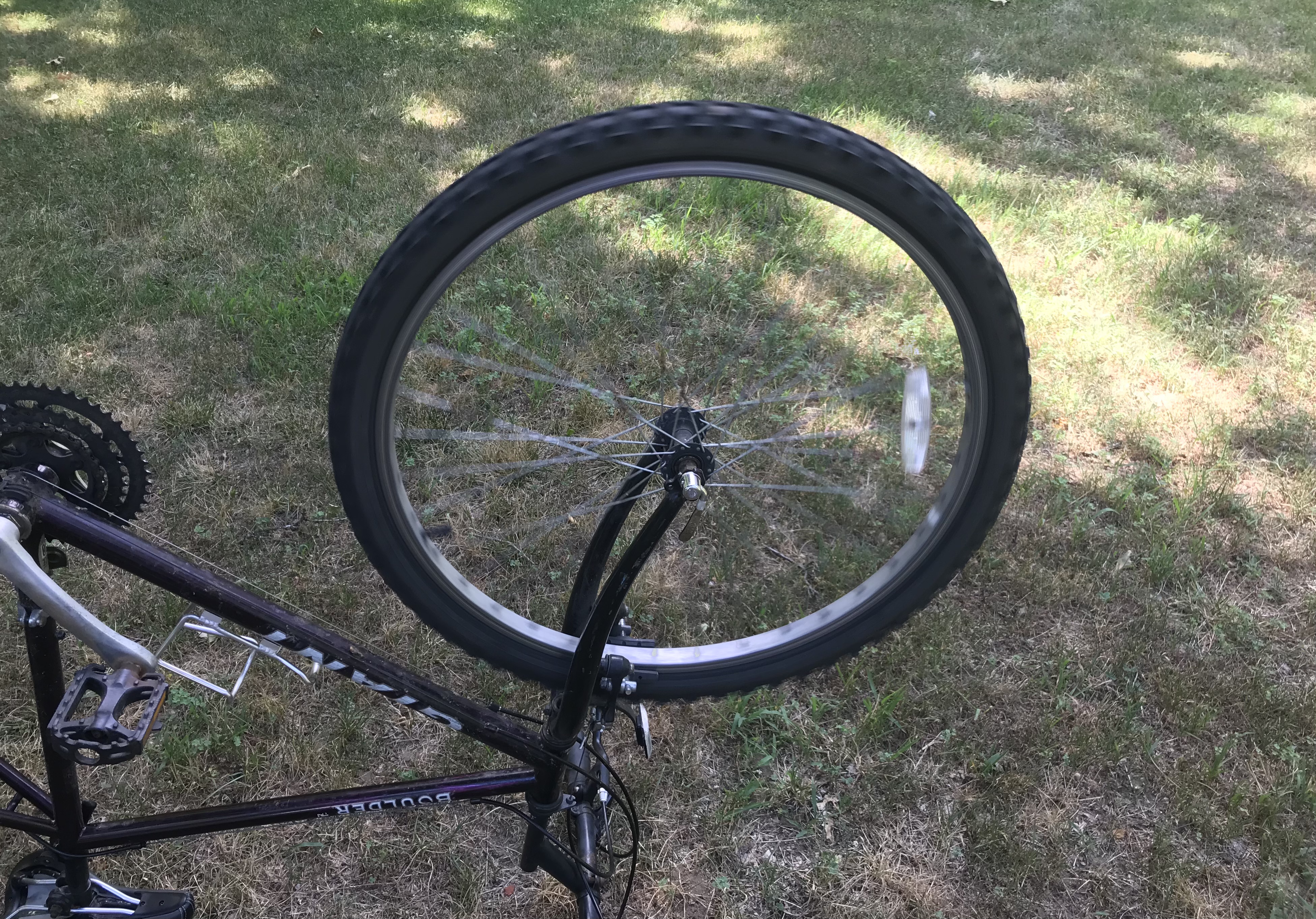
As a very simple example, consider the bike wheel in the figure below, with a moment of inertia of 10 kg m\(^2\) shown spinning at a rate of 3 rev/s. It would appear this wheel is spinning freely, but of course we know that there is some kind of friction between the axle and the wheel that is slowing it down. If we modeled this friction as torque, and said for example that the size of this torque is 1.0 Nm, we could determine how long it would take for the wheel to stop using the equation above.

Solution

Following the problem solving framework from an earlier section of this textbook:

Translate: We will use the following variables:
\[\omega_i = 3\text{ rev/s } = 18.8\text{ rad/s },\quad \omega_j=0,\quad \Delta t =?, \quad I = 10 \text{ kg m}^2,\quad \tau=1.0\text{ Nm }.\]
Notice a few things - first, we have converted the initial speed from revolutions per second to radians per second. Although this is not always necessary, here it's important because the torque is in units of Newton-meters, which is SI. We've set the final speed to be zero, specified our time as the unknown variable, and set our torque equal to the variable \(\tau\) (if you are worried about the sign of that variable - good catch! We'll deal with that later...). Finally, we've indicated that the direction of the torque is in the z-coordinate, and that it is negative. Choosing the z-coordinate along the axis of rotation is rather arbitrary, but a common standard. We've included a negative sign to be clear we know it's slowing down relative to the direction of the angular momentum, which is in the direction of \(\vec{\omega}\) here, since \(\vec{L}=I\vec{\omega}\).
Model: We are going to use conservation of angular momentum - specifically the equation from above, \(\vec{\tau}=\frac{\Delta \vec{L}}{\Delta t}\).
Solve: First, we specify the given equation into it's component form. Since the initial speed is just along the axis of rotation, let's take that to be the z-direction and then we just need that component::
\[\vec{\tau}=\frac{\Delta \vec{L}}{\Delta t} \rightarrow \tau_z=\frac{L_{zf}-L_{zi}}{\Delta t}.\]
Now we plug in the variables above, and solve for the unknown:
\[\rightarrow -\tau = \frac{0 - I\omega_i}{\Delta t} \rightarrow \Delta t=\frac{I\omega_i}{\tau}\simeq 188\text{ s}.\]
Notice in this step we have indicated that the torque (in the z-direction) should be negative - that's because we declared that the angular velocity \(\omega_i\) was positive, so if the object is going to loose momentum, the torque has to be negative. That also cancelled the negative sign on the other side of the equation.
Check: There is not a lot we can do to check this, but we can easily imagine a bike wheel spinning this fast might take ~3 minutes to slow down to a stop!