13.1: Orbits

Types of Orbits Under an Inverse-Square Force

Consider a system formed by two particles (or two perfect, rigid spheres) interacting only with each other, through their gravitational attraction. Conservation of the total momentum tells us that the center of mass of the system is either at rest or moving with constant velocity. Let us assume that one of the objects has a much greater mass, \(M\), than the other, so that, for practical purposes, its center coincides with the center of mass of the whole system. This is not a bad approximation if what we are interested in is, for instance, the orbit of a planet around the sun. The most massive planet, Jupiter, has only about 0.001 times the mass of the sun.

Accordingly, we will assume that the more massive object does not move at all (by working in its center of mass reference frame, if necessary—note that, by our assumptions, this will be an inertial reference frame to a good approximation), and we will be concerned only with the motion of the less massive object under the force \(F = GMm/r^2\), where \(r\) is the distance between the centers of the two objects. Since this force is always pulling towards the center of the more massive object (it is what is often called a central force), its torque around that point is zero, and therefore the angular momentum, \(\vec L\), of the less massive body around the center of mass of the system is constant. This is an interesting result: it tells us, for instance, that the motion is confined to a plane, the same plane that the vectors \(\vec r\) and \(\vec v\) defined initially, since their cross-product cannot change.

In spite of this simplification, the calculation of the object’s trajectory, or orbit, requires some fairly advanced mathematical techniques, except for the simplest case, which is that of a circular orbit of radius \(R\). Note that this case requires a very precise relationship to hold between the object’s velocity and the orbit’s radius, which we can get by setting the force of gravity equal to the centripetal force:

\[ \frac{G M m}{R^{2}}=\frac{m v^{2}}{R} \label{eq:10.11} .\]

So, if we want to, say, put a satellite in a circular orbit around a central body of mass \(M\) and at a distance \(R\) from the center of that body, we can do it, but only provided we give the satellite an initial velocity \(v=\sqrt{G M / R}\) in a direction perpendicular to the radius. But what if we were to release the satellite at the same distance \(R\), but with a different velocity, either in magnitude or direction? Too much speed would pull it away from the circle, so the distance to the center, \(r\), would temporarily increase; this would increase the system’s potential energy and accordingly reduce the satellite’s velocity, so eventually it would get pulled back; then it would speed up again, and so on.

You may experiment with this kind of thing yourself using the PhET demo at this link:

https://phet.colorado.edu/en/simulation/gravity-and-orbits

You will find that, as long as you do not give the satellite—or planet, in the simulation—too much speed (more on this later!) the orbit you get is, in fact, a closed curve, the kind of curve we call an ellipse. I have drawn one such ellipse for you in Figure \(\PageIndex{3}\).

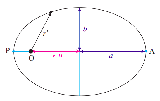
Figure \(\PageIndex{3}\): An elliptical orbit. The semimajor axis is \(a\), the semiminor axis is \(b\), and the eccentricity \(e=\sqrt{1-b^{2} / a^{2}}\) = 0.745 in this case.. The “center of attraction” (the sun, for instance, in the case of a planet’s or comet’s orbit) is at the point O.

As a geometrical curve, any ellipse can be characterized by a couple of numbers, \(a\) and \(b\), which are the lengths of the semimajor and semiminor axes, respectively. These lengths are shown in the figure. Alternatively, one could specify \(a\) and a parameter known as the eccentricity, denoted by \(e\) (do not mistake this “\(e\)” for the coefficient of restitution of Chapter 4!), which is equal to \(e=\sqrt{1-b^{2} / a^{2}}\). If \(a\) = \(b\), or \(e\) = 0, the ellipse becomes a circle.

The most striking feature of the elliptical orbits under the influence of the \(1/r^2\) gravitational force is that the “central object” (the sun, for instance, if we are interested in the orbit of a planet, asteroid or comet) is not at the geometric center of the ellipse. Rather, it is at a special point called the focus of the ellipse (labeled “O” in the figure, since that is the origin for the position vector of the orbiting body). There are actually two foci, symmetrically placed on the horizontal (major) axis, and the distance of each focus to the center of the ellipse is given by the product \(ea\), that is, the product of the eccentricity and the semimajor axis. (This explains why the “eccentricity” is called that: it is a measure of how “off-center” the focus is.)

For an object moving in an elliptical orbit around the sun, the distance to the sun is minimal at a point called the perihelion, and maximal at a point called the aphelion. Those points are shown in the figure and labeled “P” and “A”, respectively. For an object in orbit around the earth, the corresponding terms are perigee and apogee; for an orbit around some unspecified central body, the terms periapsis and apoapsis are used. There is some confusion as to whether the distances are to be measured from the surface or from the center of the central body; here I will assume they are all measured from the center, in which case the following relationships follow directly from Figure \(\PageIndex{3}\):

\begin{align}
r_{\max } &=(1+e) a \nonumber \\
r_{\min } &=(1-e) a \nonumber \\
r_{\min }+r_{\max } &=2 a \nonumber \\
e &=\frac{r_{\max }-r_{\min }}{2 a} \label{eq:10.12} .
\end{align}

The ellipse I have drawn in Figure \(\PageIndex{3}\) is actually way too eccentric to represent the orbit of any planet in the solar system (although it could well be the orbit of a comet). The planet with the most eccentric orbit is Mercury, and that is only \(e\) = 0.21. This means that \(b\) = 0.978\(a\), an almost imperceptible deviation from a circle. I have drawn the orbit to scale in Figure \(\PageIndex{4}\), and as you can see the only way you can tell it is an ellipse is, precisely, because the sun is not at the center.

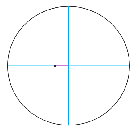
Figure \(\PageIndex{4}\): Orbit of Mercury, with the sum approximately to scale

Since an ellipse has only two parameters, and we have two constants of the motion (the total energy, \(E\), and the angular momentum, \(L\)), we should be able to determine what the orbit will look like based on just those two quantities. Under the assumption we are making here, that the very massive object does not move at all, the total energy of the system is just

\[ E=\frac{1}{2} m v^{2}-\frac{G M m}{r} \label{eq:10.13} .\]

For a circular orbit, the radius \(R\) determines the speed (as per Equation (\ref{eq:10.11})), and hence the total energy, which is easily seen to be \(E=-\frac{G M m}{2 R}\). It turns out that this formula holds also for elliptical orbits, if one substitutes the semimajor axis \(a\) for \(R\):

\[ E=-\frac{G M m}{2 a} \label{eq:10.14} .\]

Note that the total energy (\ref{eq:10.14}) is negative. This means that we have a bound orbit, by which I mean, a situation where the orbiting object does not have enough kinetic energy to fly arbitrarily far away from the center of attraction. Indeed, since \(U^G \rightarrow 0\) as \(r \rightarrow \infty\), you can see from Equation (\ref{eq:10.13}) that if the two objects could be infinitely far apart, the total energy would eventually have to be positive, for any nonzero speed of the lighter object. So, if \(E < 0\), we have bound orbits, which are ellipses (of which a circle is a special case), and conversely, if \(E > 0\) we have “unbound” trajectories, which turn out to be hyperbolas⁴. These trajectories just pass near the center of attraction once, and never return.

The special borderline case when \(E\) = 0 corresponds to a parabolic trajectory. In this case, the particle also never comes back: it has just enough kinetic energy to make it “to infinity,” slowing down all the while, so \(v \rightarrow 0\) as \(r \rightarrow \infty\). The initial speed necessary to accomplish this, starting from an initial distance \(r_i\), is usually called the “escape velocity” (although it really should be called the escape speed), and it is found by simply setting Equation (\ref{eq:10.13}) equal to zero, with \(r = r_i\), and solving for \(v\):

\[ v_{e s c}=\sqrt{\frac{2 G M}{r_{i}}} \label{eq:10.15} .\]

In general, you can calculate the escape speed from any initial distance \(r_i\) to the central object, but most often it is calculated from its surface. Note that \(v_{esc}\) does not depend on the mass of the lighter object (always assuming that the heavier object does not move at all). The escape velocity from the surface of the earth is about 11 km/s, or 1.1×10⁴ m/s; but this alone would not be enough to let you leave the attraction of the sun behind. The escape speed from the sun starting from a point on the earth’s orbit is 42 km/s.

To summarize all of the above, suppose you are trying to put something in orbit around a much more massive body, and you start out a distance \(r\) away from the center of that body. If you give the object a speed smaller than the escape speed at that point, the result will be \(E\) < 0 and an elliptical orbit (of which a circle is a special case, if you give it the precise speed \(v=\sqrt{G M / r}\) in the right direction). If you give it precisely the escape speed (\ref{eq:10.15}), the total energy of the system will be zero and the trajectory of the object will be a parabola; and if you give it more speed than \(v_{esc}\), the total energy will be positive and the trajectory will be a hyperbola. This is illustrated in Figure \(\PageIndex{5}\) below.

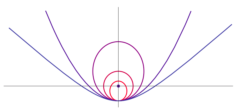
Figure \(\PageIndex{5}\): Possible trajectories for an object that is “released” with a sideways velocity at the lowest point in the figure, under the gravitational attraction of a large mass represented by the black circle. Each trajectory corresponds to a different value of the object’s initial kinetic energy: if \(K_{circ}\) is the kinetic energy needed to have a circular orbit through the point of release, the figure shows the cases \(K_i = 0.5K_{circ}\) (small ellipse), \(K_i = K_{circ}\) (circle), \(K_i = 1.5K_{circ}\) (large ellipse), \(K_i = 2K_{circ}\) (escape velocity, parabola), and \(K_i = 2.5K_{circ}\) (hyperbola).

Note that all the trajectories shown in Figure \(\PageIndex{5}\) have the same potential energy at the “point of release” (since the distance from that point to the center of attraction is the same for all), so increasing the kinetic energy at that point also means increasing the total energy (\ref{eq:10.13}) (which is constant throughout). So the picture shows different orbits in order of increasing total energy.

For a given total energy, the total angular momentum does not change the fundamental nature of the orbit (bound or unbound), but it can make a big difference on the orbit’s shape. Generally speaking, for a given energy the orbits with less angular momentum will be “narrower,” or “more squished” than the ones with more angular momentum, since a smaller initial angular momentum at the point of insertion means a smaller sideways velocity component. In the extreme case of zero initial angular momentum (no sideways velocity at all), the trajectory, regardless of the total energy, reduces to a straight line, either straight towards or straight away from the center of attraction.

For elliptical orbits, one can prove the result

\[ e=\sqrt{1-\frac{L^{2}}{a G M m^{2}}} \label{eq:10.16} \]

which shows how the eccentricity increases as \(L\) decreases, for a given value of \(a\) (which is to say, for a given total energy). I should at least sketch how to obtain this result, since it is a variant of a procedure that you may have to use for some homework problems this semester. You start by writing the angular momentum as \(L = mr_Pv_P\) (or \(mr_Av_A\)), where \(A\) and \(P\) are the special points shown in Figure \(\PageIndex{3}\), where \(\vec v\) and \(\vec r\) are perpendicular. Then, you note that \(r_P = r_{min} = (1 − e)a\) (or, alternatively, \(r_A = r_{max} = (1 + e)a\)), so \(v_P = L/[m(1− e)a]\). Then substitute these expressions for \(r_P\) and \(v_P\) in Equation (\ref{eq:10.13}), set the result equal to the total energy (\ref{eq:10.14}), and solve for \(e\).

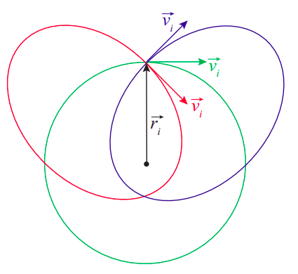
Figure \(\PageIndex{6}\): Effect of the "angle of insertion" on the orbit.

Figure \(\PageIndex{6}\) illustrates the effect of varying the angular momentum, for a given energy. All the initial velocity vectors in the figure have the same magnitude, and the release point (with position vector \(\vec r_i\)) is the same for all the orbits, so they all have the same energy; indeed, you can check that the semimajor axis of the two ellipses is the same as the radius of the circle, as required by Equation (\ref{eq:10.14}). The difference between the orbits is their total angular momentum. The green orbit has the maximum angular momentum possible at the given energy, since the green velocity vector is perpendicular to \(\vec r_i\). Note that this (maximizing \(L\) for a given \(E\) < 0) always results in a circle, in agreement with Equation (\ref{eq:10.15}): the eccentricity is zero when \( L=L_{c i r c} \equiv \sqrt{a G M m^{2}}\), which is the largest value of \(L\) allowed in Equation (\ref{eq:10.15}).

For the other two orbits, \(\vec v_i\) and \(\vec r_i\) make angles of 45\(^{\circ}\) and 135\(^{\circ}\), and so the angular momentum \(L\) has magnitude \(L=L_{\text {circ}} \sin 45^{\circ}=L_{\text {circ}} / \sqrt{2}\). The result are the red and blue ellipses, with eccentricities \(e=\sqrt{1-\sin ^{2}\left(45^{\circ}\right)}\) = 0.707.

---

⁴There is apparently a way to describe a hyperbola as an ellipse with eccentricity \(e\) > 1, but I’m definitely not going to go there.

---