13.2: Kepler's Laws

Kepler's Laws

The first great success of Newton’s theory was to account for the results that Johannes Kepler had extracted from astronomical data on the motion of the planets around the sun. Kepler had managed to find a number of regularities in a mountain of data (most of which were observations by his mentor, the Danish astronomer Tycho Brahe), and expressed them in a succinct way in mathematical form. These results have come to be known as Kepler’s laws, and they are as follows:

1. The planets move around the sun in elliptical orbits, with the sun at one focus of the ellipse
2. (Law of areas) A line that connects the planet to the sun (the planet’s position vector) sweeps equal areas in equal times.
3. The square of the orbital period of any planet is proportional to the cube of the semimajor axis of its orbit (the same proportionality constant holds for all the planets).

I have discussed the first “law” at length in the previous section, and also pointed out that the math necessary to prove it is far from trivial. The second law, on the other hand, while it sounds complicated, turns out to be a straightforward consequence of the conservation of angular momentum. To see what it means, consider Figure \(\PageIndex{7}\).

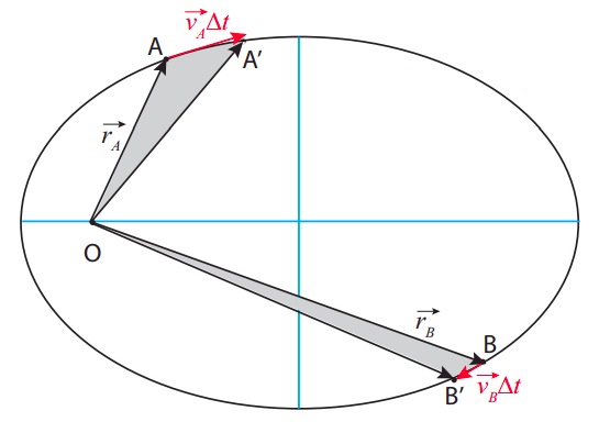
Figure \(\PageIndex{7}\): Illustrating Kepler’s law of areas. The two gray “curved triangles” have the same area, so the particle must take the same time to go from A to A\(^{\prime}\) as it does to go from B to B\(^{\prime}\).

Suppose that, at some time \(t_A\), the particle is at point A, and a time \(\Delta t\) later it has moved to A\(^{\prime}\). The area “swept” by its position vector is shown in grey in the figure, and Kepler’s second law states that it must be the same, for the same time interval, at any point in the trajectory; so, for instance, if the particle starts out at B instead, then in the same time interval \(\Delta t\) it will move to a point B\(^{\prime}\) such that the area of the “curved triangle” OBB\(^{\prime}\) equals the area of OAA\(^{\prime}\).

Qualitatively, this means that the particle needs to move more slowly when it is farther from the center of attraction, and faster when it is closer. Quantitatively, this actually just means that its angular momentum is constant! To see this, note that the straight distance from A to A\(^{\prime}\) is the displacement vector \(\Delta \vec{r}_A\), which, for a sufficiently short interval \(\Delta t\), will be approximately equal to \(\vec{v}_A \Delta t\). Again, for small \(\Delta t\), the area of the curved triangle will be approximately the same as that of the straight triangle OAA\(^{\prime}\). It is a well-known result in trigonometry that the area of a triangle is equal to 1/2 the product of the lengths of any two of its sides times the sine of the angle they make. So, if the two triangles in the figures have the same areas, we must have

\[ \left|\vec{r}_{A}\right|\left|\vec{v}_{A}\right| \Delta t \sin \theta_{A}=\left|\vec{r}_{B}\right|\left|\vec{v}_{B}\right| \Delta t \sin \theta_{B} \label{eq:10.17} \]

and we recognize here the condition \(\left|\vec{L}_{\boldsymbol{A}}\right|=\left|\vec{L}_{B}\right|\), which is to say, conservation of angular momentum. (Once the result is established for infinitesimally small \(\Delta t\), we can establish it for finite-size areas by using integral calculus, which is to say, in essence, by breaking up large triangles into sums of many small ones.)

As for Kepler’s third result, it is easy to establish for a circular orbit, and definitely not easy for an elliptical one. Let us call \(T\) the orbital period, that is, the time it takes for the less massive object to go around the orbit once. For a circular orbit, the angular velocity \(\omega\) can be written in terms of \(T\) as \(\omega = 2\pi / T\), and hence the regular speed \(v = R\omega = 2\pi R/T\). Substituting this in Equation (\ref{eq:10.11}), we get \(GM/R^2 = 4\pi^{2}R/T^{2}\), which can be simplified further to read

\[ T^{2}=\frac{4 \pi^{2}}{G M} R^{3} \label{eq:10.18} .\]

Again, this turns out to work for an elliptical orbit if we replace \(R\) by \(a\).

Note that the proportionality constant in Equation (\ref{eq:10.18}) depends only on the mass of the central body. For the solar system, that would be the sun, of course, and then the formula would apply to any planet, asteroid, or comet, with the same proportionality constant. This gives you a quick way to calculate the orbital period of anything orbiting the sun, if you know its distance (or vice-versa), based on the fact that you know what these quantities are for the Earth.

More generally, suppose you have two planets, 1 and 2, both orbiting the same star, at distances \(R_1\) and \(R_2\), respectively. Then their orbital periods \(T_1\) and \(T_2\) must satisfy \(T_{1}^{2}=\left(4 \pi^{2} / G M\right) R_{1}^{3}\) and \( T_{2}^{2}=\left(4 \pi^{2} / G M\right) R_{2}^{3} \). Divide one equation by the other, and the proportionality constant cancels, so you get

\[ \left(\frac{T_{2}}{T_{1}}\right)^{2}=\left(\frac{R_{2}}{R_{1}}\right)^{3} \label{eq:10.19} .\]

From this, some simple manipulation gives you

\[ T_{2}=T_{1}\left(\frac{R_{2}}{R_{1}}\right)^{3 / 2} \label{eq:10.20} .\]

Note you can express \(R_1\) and \(R_2\) in any units you like, as long as you use the same units for both, and similarly \(T_1\) and \(T_2\). For instance, if you use the Earth as your reference “planet 1,” then you know that \(T_1\) = 1 (in years), and \(R_1\) = 1, in AU (an AU, or “astronomical unit,” is the distance from the Earth to the sun). A hypothetical planet at a distance of 4 AU from the sun should then have an orbital period of 8 Earth-years, since \(4^{3 / 2}=\sqrt{4^{3}}=\sqrt{64}=8\).

A formula just like (\ref{eq:10.18}), but with a different proportionality constant, would apply to the satellites of any given planet; for instance, the myriad of artificial satellites that orbit the Earth. Again, you could introduce a “reference satellite” labeled 1, with known period and distance to the Earth (the moon, for instance?), and derive again the result (\ref{eq:10.20}), which would allow you to get the period of any other satellite, if you knew how its distance to the earth compares to the moon’s (or, conversely, the distance at which you would need to place it in order to get a desired orbital period).

For instance, suppose I want to place a satellite on a “geosynchronous” orbit, meaning that it takes 1 day for it to orbit the Earth. I know the moon takes 29 days, so I can write Equation (\ref{eq:10.20}) as \(1 = 29(R_2/R_1)^{3/2}\), or, solving it, \(R_2/R_1 = (1/29)^{2/3} = 0.106\), meaning the satellite would have to be approximately 1/10 of the Earth-moon distance from (the center of) the Earth.

In hindsight, it is somewhat remarkable that Kepler’s laws are as accurate, for the solar system, as they turned out to be, since they can only be mathematically derived from Newton’s theory by making a number of simplifying approximations: that the sun does not move, that the gravitational force of the other planets has no effect on each planet’s orbit, and that the planets (and the sun) are perfect spheres, for instance. The first two of these approximations work as well as they do because the sun is so massive; the third one works because the sizes of all the objects involved (including the sun) are much smaller than the corresponding orbits. Nevertheless, Newton’s work made it clear that Kepler’s laws could only be approximately valid, and scientists soon set to work on developing ways to calculate the corrections necessary to deal with, for instance, the trajectories of comets or the orbit of the moon.

Of the main approximations I have listed above, the easiest one to get rid of (mathematically) is the first one, namely, that the sun does not move. Instead, what one finds is that, as long as the sun and the planet are still treated as an isolated system, they will both revolve around the system’s center of mass. Of course, the sun’s motion (a slight “wobble”) is very small, but not completely negligible. You can even see it in the simulation I mentioned earlier, at

phet.colorado.edu/en/simulation/gravity-and-orbits.

What is much harder to deal with, mathematically, is the fact that none of the planets in the solar system actually forms an isolated system with the sun, since all the planets are really pulling gravitationally on each other all the time. Particularly, Jupiter and Saturn have a non-negligible influence on each other’s orbits, and on the orbits of every other planet, which can only be perceived over centuries. Basically, the orbits still look like ellipses to a very good degree, but the ellipses rotate very, very slowly (so they fail to exactly close in on themselves). This effect, known as orbital precession, is most dramatic for Mercury, where the ellipse’s axes rotate by more than one degree per century.

Nevertheless, the Newtonian theory is so accurate, and the calculation techniques developed over the centuries so sophisticated, that by the early 20th century the precession of the orbits of all planets except Mercury had been calculated to near exact agreement with the best observational data. The unexplained discrepancy for Mercury amounted only to 43 seconds of arc per century, out of 5600 (an error of only 0.8%). It was eventually resolved by Einstein’s general theory of relativity.