
20.1: Motion on a Circle (Or Part of a Circle)
- Page ID
- 63273

The last example of motion in two dimensions that I will consider in this chapter is motion on a circle. There are many examples of circular (or near-circular) motion in nature, particularly in astronomy (as we shall see in a later chapter, the orbits of most planets and many satellites are very nearly circular). There are also many devices that we use all the time that involve rotating or spinning objects (wheels, gears, turntables, turbines...). All of these can be mathematically described as collections of particles moving in circles.
In this section, I will first introduce the concept of centripetal force, which is the force needed to bend an object’s trajectory into a circle (or an arc of a circle), and then I will also introduce a number of quantities that are useful for the description of circular motion in general, such as angular velocity and angular acceleration. The dynamics of rotational motion (questions having to do with rotational energy, and a new important quantity, angular momentum) will be the subject of Chapter 23.
Centripetal Acceleration and Centripetal Force
As you know by now, the law of inertia states that, in the absence of external forces, an object will move with constant speed on a straight line. A circle is not a straight line, so an object will not naturally follow a circular path unless there is a force acting on it.
Another way to see this is to go back to the definition of acceleration. If an object has a velocity vector \(\vec v(t)\) at the time \(t\), and a different velocity vector \(\vec v(t + \Delta t)\) at the later time \(t + \Delta t\), then its average acceleration over the time interval \(\Delta t\) is the quantity \(\vec v_{av} = (\vec v(t + \Delta t) − \vec v(t))/ \Delta t\). This is nonzero even if the speed does not change (that is, even if the two velocity vectors have the same magnitude), as long as they have different directions, as you can see from Figure \(\PageIndex{1}\) below. Thus, motion on a circle (or an arc of a circle), even at constant speed, is accelerated motion, and, by Newton’s second law, accelerated motion requires a force to make it happen.
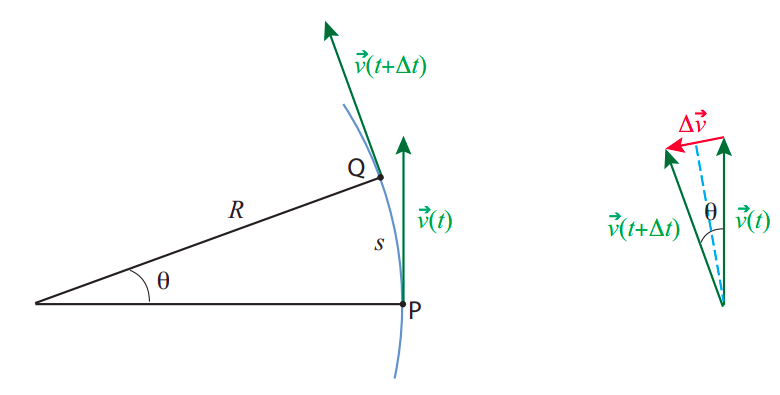
We can find out how large this acceleration, and the associated force, have to be, by applying a little geometry and trigonometry to the situation depicted in Figure \(\PageIndex{1}\). Here a particle is moving along an arc of a circle of radius \(R\), so that at the time \(t\) it is at point P and at the later time \(t+ \Delta t\) it is at point Q. The length of the arc between P and Q (the distance it has traveled) is \(s = R\theta\), where the angle \(\theta\) is understood to be in radians. I have assumed the speed to be constant, so the magnitude of the velocity vector, \(v\), is just equal to the ratio of the distance traveled (along the circle), to the time elapsed: \(v = s/ \Delta t\). Combining these two expressions, we have a relationship for the angle in the figure:
\[\theta=\frac{s}{R}=\frac{v \Delta t}{R}.\]
Now, consider the second picture in the figure above. It shows the change of the velocity vector from \(\vec{v}(t)\) to \(\vec{v}(t+\Delta t)\), and it should be pretty easy to convince yourself that the angle \(\theta\) between these two vectors is the same as in the left figure. Now, unlike the "definition of the angle" \(\theta=s/r\) relationship we used above, this is a real triangle (\(\Delta\vec{v}\) is a straight line), but we can say approximately the same thing is true,
\[\theta=\frac{\Delta v}{v(t)}.\]
Since these two are relationships for the angle (which should be the same), we can set them equal to each other:
\[\frac{v \Delta t}{R}=\frac{\Delta v}{v(t)}\rightarrow \frac{\Delta v}{\Delta t}=\frac{v^2}{R}.\]
In the last step we have solved for the change in velocity over the change in time, which is simply the acceleration,
\[a_c=\frac{v^2}{R}.\]
This acceleration is called the centripetal acceleration, which is why I have denoted it by the symbol \(a_c\). The reason for that name is that it is always pointing towards the center of the circle. You can kind of see this from Figure \(\PageIndex{1}\): if you take the vector \(\Delta \vec v\) shown there, and move it (without changing its direction, so it stays ‘parallel to itself”) to the midpoint of the arc, halfway between points P and Q, you will see that it does point almost straight to the center of the circle. (A more mathematically rigorous proof of this fact, using calculus, will be presented later in this section.)
The force \(\vec F_c\) needed to provide this acceleration is called the centripetal force, and by Newton’s second law it has to satisfy \(\vec F_c = m\vec a_c\). Thus, the centripetal force has magnitude
\[ F_{c}=m a_{c}=\frac{m v^{2}}{R} \label{eq:8.28} \]
and, like the acceleration \(\vec a_c\), is always directed towards the center of the circle.
Physically, the centripetal force \(F_c\), as given by Equation (\ref{eq:8.28}), is what it takes to bend the trajectory so as to keep it precisely on an arc of a circle of radius \(R\) and with constant speed \(v\). Note that, since \(\vec F_c\) is always perpendicular to the displacement (which, over any short time interval, is essentially tangent to the circle), it does no work on the object, and therefore (by Equation (10.2.7)) its kinetic energy does not change, so \(v\) does indeed stay constant when the centripetal force equals the net force. Note also that “centripetal” is just a job description: it is not a new type of force. In any given situation, the role of the centripetal force will be played by one of the forces we are already familiar with, such as the tension on a rope (or an appropriate component thereof) when you are swinging an object in a horizontal circle, or gravity in the case of the moon or any other satellite.
At this point, if you have never heard about the centripetal force before, you may be feeling a little confused, since you almost certainly have heard, instead, about a so-called centrifugal force that tends to push spinning things away from the center of rotation. In fact, however, this “centrifugal force” does not really exist: the “force” that you may feel pushing you towards the outside of a curve when you ride in a vehicle that makes a sharp turn is really nothing but your own inertia—your body “wants” to keep moving on a straight line, but the car, by bending its trajectory, is preventing it from doing so. The impression that you get that you would fly radially out, as opposed to along a tangent, is also entirely due to the fact that the reference frame you are in (the car) is continuously changing its direction of motion. Example 20.2.3 illustrates this in some detail.
On the other hand, getting a car to safely negotiate a turn is actually an important example of a situation that requires a definite centripetal force. On a flat surface (see the next section for a treatment of a banked curve!), you rely entirely on the force of static friction to keep you on the track, which can typically be modeled as an arc of a circle with some radius \(R\). So, if you are traveling at a speed \(v\), you need \(F^s = mv^2/R\). Recalling that the force of static friction cannot exceed \(\mu_sF^n\), and that on a flat surface you would just have \(F^n = F^g = mg\), you see you need to keep \(mv^2/R\) smaller than \(\mu_{s}mg\); or, canceling the mass,
\[ \frac{v^{2}}{R}<\mu_{s} g \label{eq:8.29} .\]
This is the condition that has to hold in order to be able to make the turn safely. The maximum speed is then \(v_{\max }=\sqrt{\mu_{s} g R}\), which, as you can see, will depend on the state of the road (for instance, if the road is wet the coefficient \(\mu_s\) will be smaller). The posted, recommended speed will typically take this into consideration and will be as low as it has to be to keep you safe. Notice that the left-hand side of Equation (\ref{eq:8.29}) increases as the square of the speed, so doubling your speed makes that term four times larger! Do not even think of taking a turn at 60 mph if the recommended speed is 30, and do not exceed the recommended speed at all if the road is wet or your tires are worn.
Kinematic Angular Variables
Consider a particle moving on a circle, as in Figure \(\PageIndex{2}\) below. Of course, we can just use the regular, cartesian coordinates, \(x\) and \(y\), to describe its motion. But, in a way, this is carrying around more information than we typically need, and it is also not very transparent: a value of \(x\) and \(y\) does not immediately tell us how far the object has traveled along the circle itself.
Instead, the most convenient way to describe the motion of the particle, if we know the radius of the circle, is to give the angle \(\theta\) that the position vector makes with some reference axis at any given time, as shown in Figure \(\PageIndex{2}\). If we choose the \(x\) axis as the reference, then the conversion from a description based on the radius \(R\) and the angle \(\theta\) to a description in terms of \(x\) and \(y\) is simply
\begin{align}
&x=R \cos \theta \nonumber \\
&y=R \sin \theta \label{eq:8.30}
\end{align}
so knowing the function \(\theta (t)\) we can immediately get \(x(t)\) and \(y(t)\), if we need them. (Note: in this section we are using an uppercase \(R\) for the magnitude of the position vector, to emphasize that it is a constant, equal to the radius of the circle.)
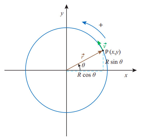
Figure \(\PageIndex{2}\): A particle moving on a circle. The position vector has length \(R\), so the \(x\) and \(y\) coordinates are \(R \cos \theta\) and \(R \sin \theta\), respectively. The conventional positive direction of motion is indicated. The velocity vector is always, as usual, tangent to the trajectory.
Although the angle \(\theta\) itself is not a vector quantity, nor a component of a vector, it is convenient to allow for the possibility that it might be negative. The standard convention is that \(\theta\) grows in the counterclockwise direction from the reference axis, and decreases in the clockwise direction. Of course, you can always get to any angle by coming from either direction, so the angle by itself does not tell you how the particle got there. Information on the direction of motion at any given time is best captured by the concept of the angular velocity, which we represent by the symbol \(\omega\) and define in a manner analogous to the way we defined the ordinary velocity: if \(\Delta \theta = \theta (t + \Delta t) − \theta (t)\) is the angular displacement over a time \(\Delta t\), then
\[ \omega=\lim _{\Delta t \rightarrow 0} \frac{\Delta \theta}{\Delta t}=\frac{d \theta}{d t} \label{eq:8.31} .\]
The standard convention is also to use radians as an angle measure in this context, so that the units of \(\omega\) will be radians per second, or rad/s. Note that the radian is a dimensionless unit, so it “disappears” from a calculation when the final result does not call for it (as in Equation (\ref{eq:8.35}) below).
For motion with constant angular velocity, we clearly will have
\[ \theta(t)=\theta_{i}+\omega\left(t-t_{i}\right) \quad \text { or } \quad \Delta \theta=\omega \Delta t \quad \text { (constant } \omega) \label{eq:8.32} \]
where \(\omega\) is positive for counterclockwise motion, and negative for clockwise. (Recall that the direction of the vector \(\vec{\omega}\) can be specified with the right hand rule, from section 7.1)
When \(\omega\) changes with time, we can introduce an angular acceleration \(\alpha\), defined, again, in the obvious way:
Then for motion with constant angular acceleration we have the formulas
Equation (\ref{eq:8.34}) completely parallel the corresponding equations for motion in one dimension that we saw in Chapter 1. In fact, of course, a circle is just a line that has been bent in a uniform way, so the distance traveled along the circle itself is simply proportional to the angle swept by the position vector \(\vec r\). As already pointed out in connection with Figure \(\PageIndex{1}\), if we expressed \(\theta\) in radians then the length of the arc corresponding to an angular displacement \(\Delta \theta\) would be
\[ s = R |\Delta \theta | \label{eq:8.35} \]
so multiplying Eqs. (\ref{eq:8.32}) or (\ref{eq:8.34}) by \(R\) directly gives the distance traveled along the circle in each case.
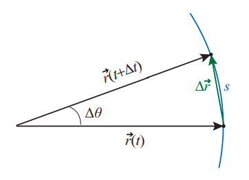
Figure \(\PageIndex{3}\) shows that, for very small angular displacements, it does not matter whether the distance traveled is measured along the circle itself or on a straight line; that is, \(s \simeq|\Delta \vec{r}|\). Dividing by \(\Delta t\), using Equation (\ref{eq:8.35}) and taking the \(\Delta t \rightarrow 0\) limit we get the following useful relationship between the angular velocity and the instantaneous speed \(v\) (defined in the ordinary way as the distance traveled per unit time, or the magnitude of the velocity vector):
\[|\vec{v}|=R|\omega| \label{eq:8.36} .\]
As we shall see later, the product \(R\alpha\) is also a useful quantity. It is not, however, equal to the magnitude of the acceleration vector, but only one of its two components, the tangential acceleration:
\[ a_{t}=R \alpha \label{eq:8.37} .\]
The sign convention here is that a positive \(a_t\) represents a vector that is tangent to the circle and points in the direction of increasing \(\theta\) (that is, counterclockwise); the full acceleration vector is equal to the sum of this vector and the centripetal acceleration vector, introduced in the previous subsection, which always points towards the center of the circle and has magnitude
\[ a_{c}=\frac{v^{2}}{R}=R \omega^{2} \label{eq:8.38} \]
(making use of Eqs. (\ref{eq:8.29}) and (\ref{eq:8.36})). These results will be formally established Chapter 22, after we introduce the vector product, although you could also verify them right now—if you are familiar enough with derivatives at this point—by using the chain rule to take the derivatives with respect to time of the components of the position vector, as given in Equation (\ref{eq:8.30}) (with \(\theta = \theta (t)\), an arbitrary function of time).
The main thing to remember about the radial and tangential components of the acceleration is that the radial component (the centripetal acceleration) is always there for circular motion, whether the angular velocity is constant or not, whereas the tangential acceleration is only nonzero if the angular velocity is changing, that is to say, if the particle is slowing down or speeding up as it turns.