22.5: Examples

After a couple of whiteboard problems, we will present a few additional examples in this section show you have to set up and solve the equations of motion for somewhat more complicated systems, and you should study them carefully.

Whiteboard Problem \(\PageIndex{1}\)

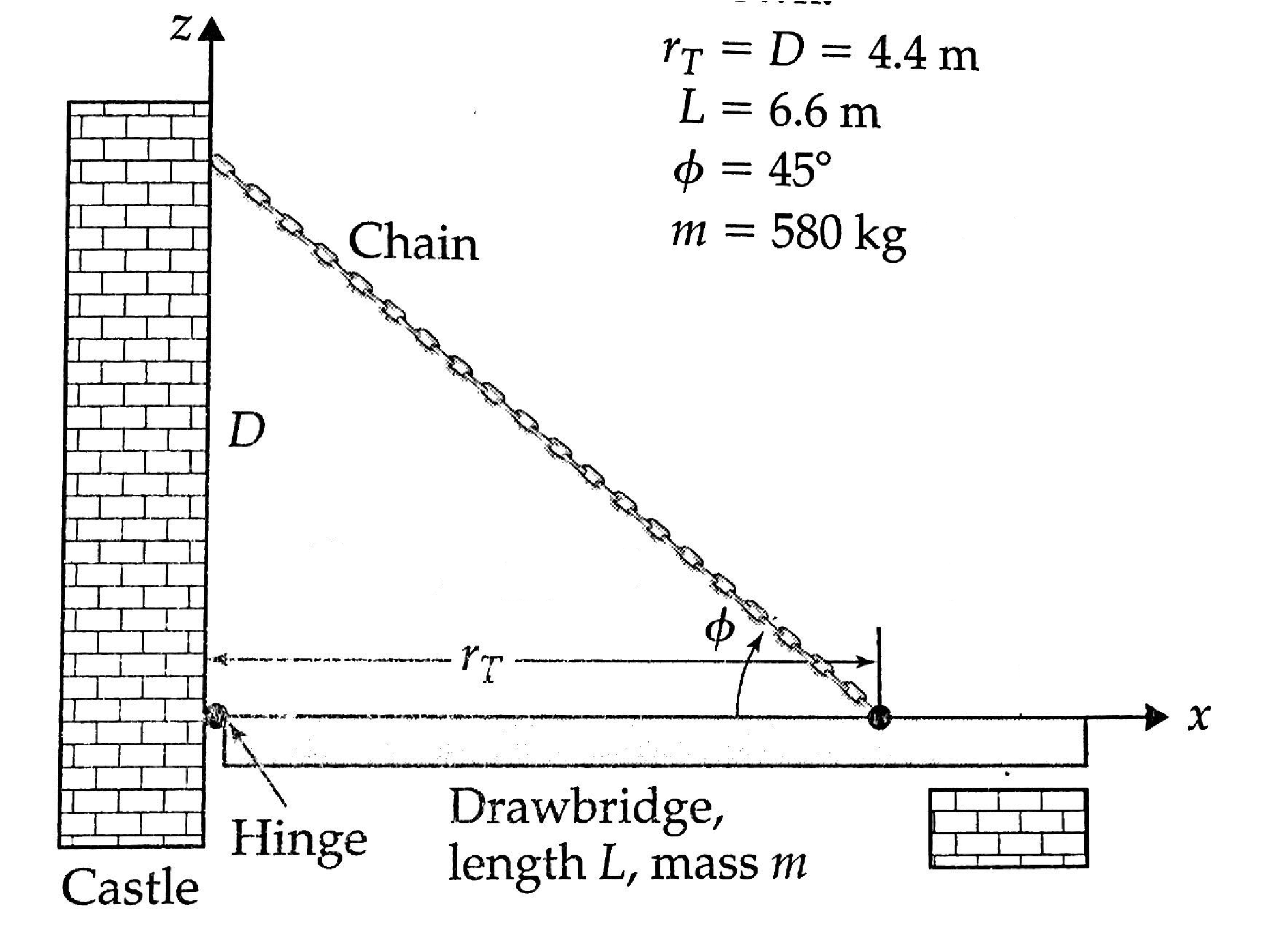
Consider the drawbridge in the figure above, which is in static equilibrium. Determine the magnitude and direction of all the forces on the bridge - tension, gravity, and the hinge.

Whiteboard Problem \(\PageIndex{2}\)

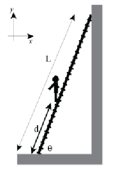
Consider a very light ladder, of length 5.0 m, placed against a wall as shown at an angle of 60\(^\circ\). The wall is smooth (no friction), but the floor is rough and the coefficient of static friction between the ladder and the floor is 0.5. A painter of mass 65 kg is standing on the ladder at a distance \(d\) from the bottom. (Hint:  Draw a free body diagram, and make sure the object appears to be in rotational equilibrium before deciding you've identified all the forces!)

1. What is the normal force exerted by the floor on the ladder? 
2. How far up the ladder \(d\) can the painter go before the ladder starts to slide? 

Whiteboard Problem \(\PageIndex{3}\)

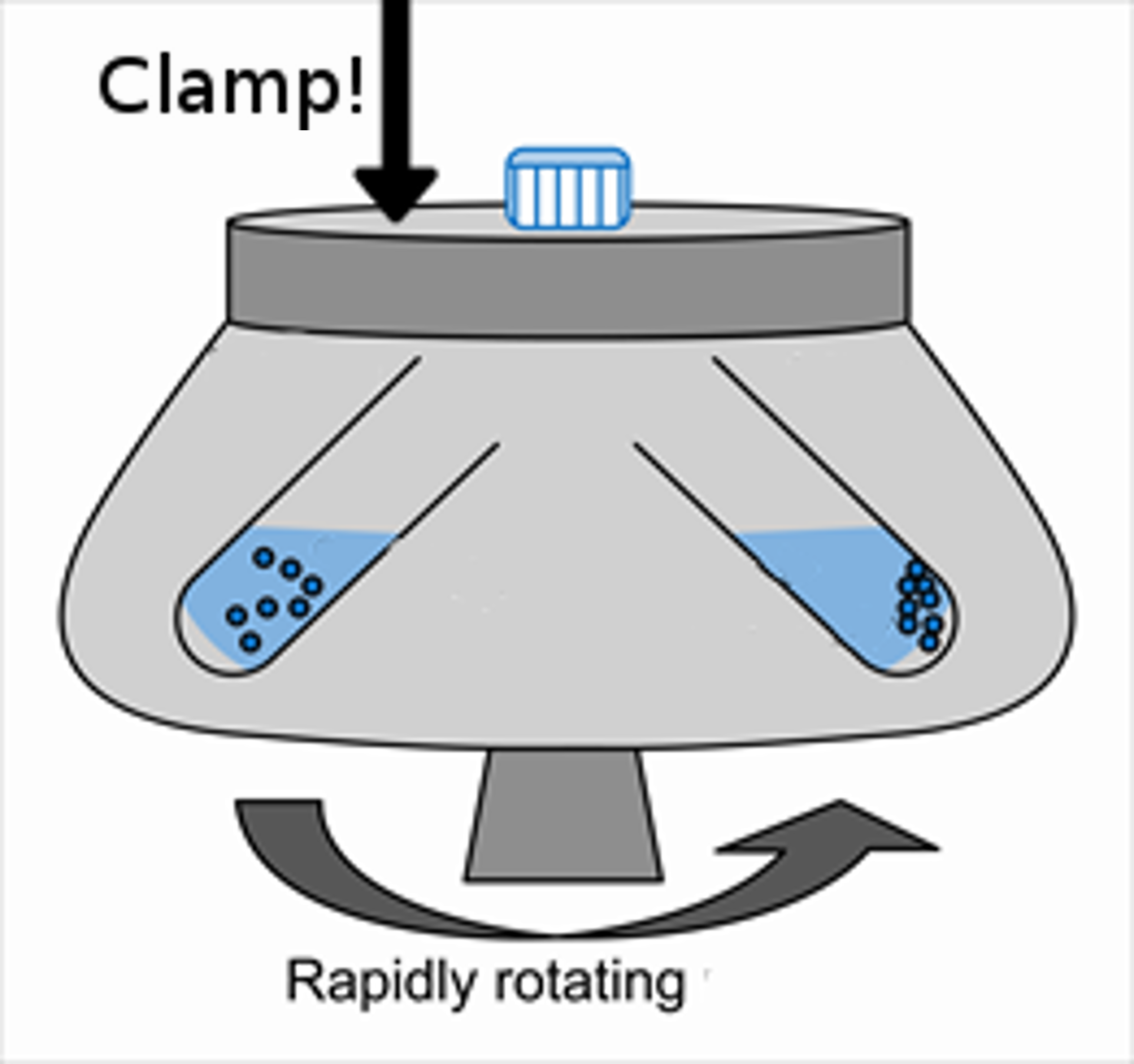
A specific centrifuge can spin at a rate of 1000 rpm.

1. What is the angular speed of this centrifuge, in radians per second?
2. The centrifuge is slowed down by applying a clamp at a distance 15 cm from the center of rotation. This clamp applies a force of 32 N to the centrifuge. What is the largest amount of torque this clamp could be exerting?
3. If the clamp exerts the largest amount of torque (which you just found), what will the angular acceleration of the centrifuge be? Take the centrifuge to be a uniform disk with radius 27 cm and total mass 4.5 kg.
4. How long will it take for this centrifuge to come to a stop?

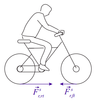
Example \(\PageIndex{4}\): Torques and forces on the wheels of an accelerating bicycle

Consider an accelerating bicycle. The rider exerts a torque on the pedals, which is transmitted to the rear wheel by the chain (possibly amplified by the gears, etc). How does this “drive” torque on the rear wheel (call it \(\tau_d\)) relate to the final acceleration of the center of mass of the bicycle?

Solution

We need first to figure out how many external forces, at a minimum, we have to deal with. As the bicycle accelerates, two things happen: the wheels (both wheels) turn faster, so there must be a net torque (clockwise in the picture, if the bicycle is accelerating to the right) on each wheel; and the center of mass of the system accelerates, so there must be a net external force on the whole system. The system is only in contact with the road, and so, as long as no slippage happens, the only external source of torques or forces on the wheels has to be the force of static friction between the tires and the road.

For the front wheel, this is in fact the only external force, and the only force of any sort that exerts a torque on that wheel (there are forces acting at the axle, but they exert no torque around the axle). Since the torque has to be clockwise, then, the force of static friction on the front wheel, applied as it is at the point of contact with the road, must point backwards, that is, opposite the direction of motion. We get then one equation of motion (of the type (22.4.13)) for that wheel:

\[ -F_{r, f t}^{s} R=I \alpha \label{eq:9.44} \]

where the subscript “ft” stands for “front tire”, and the wheel is supposed to have a radius \(R\) and moment of inertia \(I\).

For the rear wheel, we have the “drive torque” \(\tau_d\), exerted by the chain, and another torque exerted by the force of static friction, \(\vec F^s_{r,rt}\), between that tire and the road. However, now the force \(\vec F^s_{r,rt}\) needs to point forward. This is because the net external force on the whole bicycle-rider system is \(\vec{F}_{r, r t}^{s}+\vec{F}_{r, f t}^{s}\), and that has to point forward, or the center of mass could never accelerate in that direction. Since we have established that \(F^s_{r,f t}\) has to point backwards, it follows that \(F^s_{r,rt}\) needs to be larger, and in the forward direction. This means we get, for the center of mass acceleration, the equation (\(F_{net} = M a_{cm}\))

\[ F_{r, r t}^{s}-F_{r, f t}^{s}=M a_{c m} \label{eq:9.45} \]

and for the rear wheel, the torque equation

\[ F_{r, r t}^{s} R-\tau_{d}=I \alpha \label{eq:9.46} .\]

I am following the convention that clockwise torques are negative, and also that a force symbol without an arrow on top represents the magnitude of the force. If a clockwise angular acceleration is likewise negative, the condition of rolling without slipping [Equation (22.4.11)] needs to be written as

\[ a_{cm} = -R \alpha \label{eq:9.47} .\]

These are all the equations we need to relate the acceleration to \(\tau_d\). We can start by solving (\ref{eq:9.44}) for \(F^s_{r,f t}\) and substituting in (\ref{eq:9.45}), then likewise solving (\ref{eq:9.46}) for \(F^s_{r,rt}\) and substituting in (\ref{eq:9.45}). The result is

\[ \frac{I \alpha+\tau_{d}}{R}+\frac{I \alpha}{R}=M a_{c m} \label{eq:9.48} \]

then use Eq (\ref{eq:9.47}) to write \(\alpha = −a_{cm}/R\), and solve for \(a_{cm}\):

\[ a_{c m}=\frac{\tau_{d}}{M R+2 I / R} \label{eq:9.49} \]

Example \(\PageIndex{5}\): Blocks connected by rope over a pulley with non-zero mass

Consider again the setup illustrated in the figure below, but now assume that the pulley has a mass \(M\) and radius \(R\). For simplicity, leave the friction force out. What is now the acceleration of the system?

Solution

The figure below shows the setup, plus free-body diagrams for the two blocks (the vertical forces on block 1 have been left out to avoid cluttering the figure, since they are not relevant here), and an extended free-body diagram for the pulley. (You can see from the pulley diagram that there has to be another force acting on it, to balance the two forces shown. This would be a contact force at the axle, directed upwards and to the left. If this was a statics problem, I would have to include it, but since it does not exert a torque around the axis of rotation, it does not contribute to the dynamics of the system, so I have left it out as well.)

Figure \(\PageIndex{1}\)

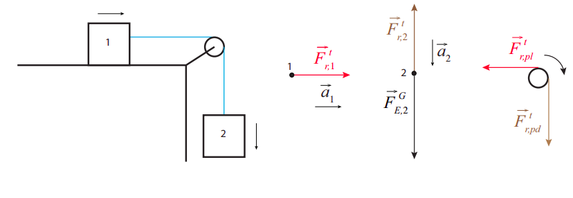
The key new feature of this problem is that the tension on the string has to have different values on either side of the pulley, because there has to be a net torque on the pulley. Hence, the leftward force on the pulley (\(F^t_{r,pl}\)) has to be smaller than the downward force (\(F^t_{r,pd}\)).

On the other hand, as long as the mass of the rope is negligible, it will still be the case that the horizontal part of the rope will pull with equal strength on block 1 and on the pulley, and similarly the vertical part of the rope will pull with equal strength on the pulley and on block 2. (To make this point clearer, I have “color-coded” these matching forces in the figure.) This means that we can write \(F^t_{r,pl} = F^t_{r,1}\) and \(F^t_{r,pd} = F^t_{r,2}\), and write the torque equation (22.4.10) for the pulley as

\[ F_{r, 1}^{t} R-F_{r, 2}^{t} R=I \alpha \label{eq:9.50} .\]

We also have \(F = ma\) for each block:

\[ F_{r, 1}^{t}=m_{1} a \label{eq:9.51} \]

\[ F_{r, 2}^{t}-m_{2} g=-m_{2} a \label{eq:9.52} \]

where I have taken \(a\) to be \(a = |\vec{a}_1| = |\vec{a}_2|\). The condition of rolling without slipping, Equation (22.4.11), applied to the pulley, gives then

\[ -R \alpha = a \label{eq:9.53} \]

since, in the situation shown, \(\alpha\) will be negative, and \(a\) has been defined as positive. Substituting Eqs. (\ref{eq:9.51}), (\ref{eq:9.52}), and (\ref{eq:9.53}) into (\ref{eq:9.50}), we get

\[ m_{1} a R-\left(m_{2} g-m_{2} a\right) R=-\frac{I a}{R} \label{eq:9.54} \]

which is easily solved for \(a\):

\[ a=\frac{m_{2} g}{m_{1}+m_{2}+I / R^{2}} \label{eq:9.55} .\]

If you look at the structure of this equation, it all makes sense. The numerator is the force of gravity on block 2, which is, ultimately, the force responsible for setting the whole thing in motion. The denominator is, essentially, the inertia of the system: ordinary inertia for the blocks, and rotational inertia for the pulley. Note further that, if we treat the pulley as a flat, homogeneous disk of mass \(M\), then \(I = \frac{1}{2}MR^2\), and the denominator of (\ref{eq:9.55}) becomes just \(m_1 + m_2 + M/2\).