23.3: Pendulums

The Simple Pendulum

Besides masses on springs, pendulums are another example of a system that will exhibit simple harmonic motion, at least approximately, as long as the amplitude of the oscillations is small. The simple pendulum is just a mass (or “bob”), approximated here as a point particle, suspended from a massless, inextensible string, as in Figure \(\PageIndex{1}\).

We could analyze the motion of the bob by using the general methods introduced in Chapter 8 to deal with motion in two dimensions—breaking down all the forces into components and applying \(\vec{F}_{net} = m\vec{a}\) along two orthogonal directions—but this turns out to be complicated by the fact that both the direction of motion and the direction of the acceleration are constantly changing. Although, under the assumption of small oscillations, it turns out that simply using the vertical and horizontal directions is good enough, this is not immediately obvious, and arguably it is not the most pedagogical way to proceed.

Figure \(\PageIndex{1}\): A simple pendulum. The mass of the bob is \(m\), the length of the string is \(l\), and torques are calculated around the point of suspension O. The counterclockwise direction is taken as positive.

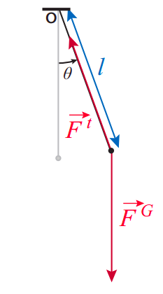
Instead, I will take advantage of the obvious fact that the bob moves on an arc of a circle, and that we have developed already in Chapter 22 a whole set of tools to deal with that kind of motion. Let us, therefore, describe the position of the pendulum by the angle it makes with the vertical, \(\theta\), and let \(\alpha = d^2 \theta /dt^2\) be the angular acceleration; we can then write the equation of motion in the form \(\tau_{net} = I\alpha\), with the torques taken around the center of rotation—which is to say, the point from which the pendulum is suspended. Then the torque due to the tension in the string is zero (since its line of action goes through the center of rotation), and \(\tau_{net}\) is just the torque due to gravity, which can be written

\[ \tau_{n e t}=-m g l \sin \theta \label{eq:11.19} .\]

The minus sign is there to enforce a consistent sign convention for \(\theta\) and \(\tau\): if, for instance, I choose counterclockwise as positive for both, then I note that when \(\theta\) is positive (pendulum to the right of the vertical), \(\tau\) is clockwise, and hence negative, and vice-versa. This is characteristic of a restoring torque, that is to say, one that will always try to push the system back to its equilibrium position (the vertical in this case).

As for the moment of inertia of the bob, it is just \(I = ml^2\) (if we treat it as just a point particle), so the equation \(\tau_{net} = I\alpha\) takes the form

\[ m l^{2} \frac{d^{2} \theta}{d t^{2}}=-m g l \sin \theta \label{eq:11.20} .\]

The mass and one factor of \(l\) cancel, and we get

\[ \frac{d^{2} \theta}{d t^{2}}=-\frac{g}{l} \sin \theta \label{eq:11.21} .\]

Equation (\ref{eq:11.21}) is an example of what is known as a differential equation. The problem is to find a function of time, \(\theta (t)\), that satisfies this equation; that is to say, when you take its second derivative the result is equal to \(−(g/l) \sin[\theta (t)]\). Such functions exist and are called elliptic functions; they are included in many modern mathematical packages, but they are still not easy to use. More importantly, the oscillations they describe, in general, are not of the simple harmonic type.

On the other hand, if the amplitude of the oscillations is small, so that the angle \(\theta\), expressed in radians, is a small number, we can make an approximation that greatly simplifies the problem, namely,

\[ \sin \theta \simeq \theta \label{eq:11.22} .\]

This is known as the small angle approximation, and requires \(\theta\) to be in radians. As an example, if \(\theta\) = 0.2 rad (which corresponds to about 11.5\(^{\circ}\)), we find \(\sin \theta\) = 0.199, to three-figure accuracy.

With this approximation, the equation to solve become much simpler:

\[ \frac{d^{2} \theta}{d t^{2}}=-\frac{g}{l} \theta \label{eq:11.23} .\]

We have, in fact, already solved an equation completely equivalent to this one in the previous section: that was equation (23.2.8) for the mass-on-a-spring system, which can be rewritten as

\[ \frac{d^{2} x}{d t^{2}}=-\frac{k}{m} x \label{eq:11.24} \]

since \(a = d^2x/dt^2\). Just like the solutions to (\ref{eq:11.24}) could be written in the form \(x(t) = A \cos(\omega t + \phi)\), with \(\omega=\sqrt{k / l}\), the solutions to (\ref{eq:11.23}) can be written as

\begin{align}
\theta(t) &=A \cos (\omega t+\phi) \nonumber \\
\omega &=\sqrt{\frac{g}{l}} \label{eq:11.25}.
\end{align}

This tells us that if a pendulum is not pulled too far away from the vertical (say, about 10\(^{\circ}\) or less) it will perform approximate simple harmonic oscillations, with a period of

\[ T=\frac{2 \pi}{\omega}=2 \pi \sqrt{\frac{l}{g}} \label{eq:11.26} .\]

This depends only on the length of the pendulum, and remains constant even as the oscillations wind down, which is why it became the basis for time-keeping devices, beginning with the invention of the pendulum clock by Christiaan Huygens in 1656. In particular, a pendulum of length \(l\) = 1 m will have a period of almost exactly 2 s, which is what gives you the familiar “tick-tock” rhythm of a “grandfather’s clock,” once per second (that is to say, once every half period).

The "Physical Pendulum"

By a “physical pendulum” one means typically any pendulum-like device for which the moment of inertia is not given by the simple expression \(I = ml^2\). This means that the mass is not concentrated into a single point-like particle a distance \(l\) away from the point of suspension; rather, for example, the bob could have a size that is not negligible compared to \(l\) (as in Figure 23.3.2a), or the “string” could have a substantial mass of its own—it could, for instance, be a chain, like in a playground swing, or a metal rod, as in most pendulum clocks.

Figure \(\PageIndex{2}\) (b) shows the special case of a thin rod of length \(l\) pivoted at one end (the distance \(d = l/2\) in this case). In both cases, there is an additional force (not shown) acting at the pivot point, to balance gravity.

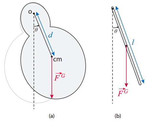
Regardless of the reason, having to deal with a distributed mass means also that one needs to use the center of mass of the system as the point of application of the force of gravity. When this is done, the motion of the pendulum can again be described by the angle between the vertical and a line connecting the point of suspension and the center of mass. If the distance between these two points is \(d\), then the torque due to gravity is \(−mgd \sin \theta\), and the only other force on the system, the force at the pivot point, exerts no torque around that point, so we can write the equation of motion in the form

\[ I \frac{d^{2} \theta}{d t^{2}}=-m g d \sin \theta \label{eq:11.27} .\]

Under the small-angle approximation, this will again lead to simple harmonic motion, only now with an angular frequency given by

\[ \omega=\sqrt{\frac{m g d}{I}} \label{eq:11.28} .\]

As an example, consider the oscillations of a uniform, thin rod of length \(l\) and mass \(m\) pivoted at one end. We then have \(I = ml^{2}/3\), and \(d = l/2\), so Equation (\ref{eq:11.28}) gives

\[ \omega=\sqrt{\frac{3 g}{2 l}} \label{eq:11.29} .\]

This is about 22% larger than the result (\ref{eq:11.25}) for a simple pendulum of the same length, implying a correspondingly shorter period.