23.4: Advanced Topics

Mass on a Spring Damped By Friction with a Surface

Consider the system depicted in Figure 23.2.1 in the presence of friction between the block and the surface. Let the coefficient of kinetic friction be \(\mu_k\) and the coefficient of static friction be \(\mu_s\). As usual, we will assume that \(\mu_s \geq \mu_k\).

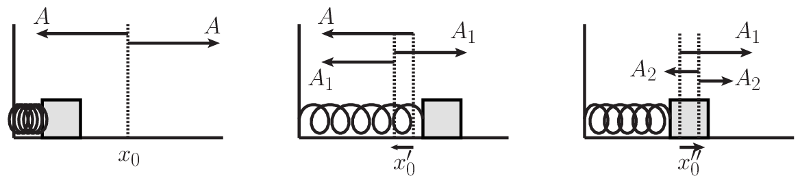
As the mass oscillates, it will experience a kinetic friction force of magnitude \(F^k = \mu_k mg\), in the direction opposite the direction of motion; that is to say, a force that changes direction every half period. As shown in section 23.2, this force does not change the frequency of the motion, but it displaces the equilibrium position in the direction of the force. Let's study this process in more detail.

First, think about that spring moving to the right - as the friction force acts on it, it shifts the position of the equilibrium, like in equation (23.2.14). We can determine the new equilibrium position using Newton's second law; we get

\[-kx_0'-\mu_kmg=0\rightarrow x_0'=-\frac{\mu_k m g}{k}.\]

(Notice we have to be careful with the signs here - when moving to the right, the friction acts the other way!) Since the equilibrium moves to the right, the actual amplitude of this motion is (see the figure) \(A_1=A-|x_0'|=A-\frac{\mu_k m g}{k}.\) Now when the block turns around, at the other maximum, during the leftward moving period the equilbrium changes again. We can find this again:

\[-kx_0''+\mu_k mg=0\rightarrow x_0''=\frac{\mu_k m g}{k}.\]

and the new amplitude is

\[A_2=A_1-|x_0''|=A-\frac{\mu_k m g}{k}-\frac{\mu_k m g}{k}=A-2\frac{\mu_k m g}{k}.\]

In other words, the amplitude after \(n\) "half swings" is \(A_n=A-n\frac{\mu_k m g}{k}\). The amplitude gets smaller and smaller each time, and in fact it vanishes for some number of these half-swings.

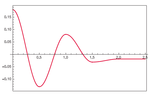
The figure below shows an example of how this would go, for the following choice of parameters: period \(T\) = 1 s, \(\mu_k\) = 0.1, and \(A\) = 0.18 m. Note that, since \(x_{0}^{\prime}\) depends only on the ratio \(m/k = 1/ \omega^2\), there is no need to specify \(m\) and \(k\) separately. We can determine the number of half-swings by just asking when the amplitude vanishes,

\[A_n=A-n\frac{\mu_k g}{\omega^2}=0\rightarrow n=\frac{A\omega^2}{\mu_k g}=4.13.\]

So that means the motion goes for 4 half-swings before stopping.

Figure \(\PageIndex{1}\): Damped oscillations.

 

Just for the record, this is not the way dissipation in simple harmonic motion is usually handled. The conventional thing is to assume a damping force that is proportional to the oscillator’s velocity. You will almost certainly see this more standard approach (which leads to a relatively simple differential equation) in some later course.

We can study this same example in a little more detail using energy. Consider the total mechanical energy of the system, \(E=\frac{1}{2}mv^2+\frac{1}{2}kx^2\). This energy does not include the friction, so we don't anticipate \(\Delta E=0\); but we can still take a time derivative of this formula to see what happens:

\[\frac{dE}{dt}=mv\frac{dv}{dt}+kx\frac{dx}{dt}=mva+kxv.\]

The first equality is taking the derivative, being careful to use the chain run on the velocity and position. The second equality is just recognizing that the derivative of velocity and position is the accleration and velocity, respectively. The resulting expression looks a bit strange, but notice that the velocity is a common term, so we can write

\[\frac{dE}{dt}=v(ma+kx).\]

The expression inside the parenthesis looks interesting, because it looks something like Newton's second law for this situation - being sure of the signs (assuming the block is moving in the positive direction) we have

\[-kx-\mu_k mg = ma\rightarrow ma+kx=-\mu_k mg.\]

Plugging this in above we finally find

\[\frac{dE}{dt}=-v\mu_k mg.\]

So the rate of energy loss is negative - exactly what we would have expected. Using a little calculus we can take this analysis further - recall that \(v=dx/dt\), so we can intergrate

\[\int_{E_i}^{E_f} dE=-\mu_k mg \int_{v_i}^{v_f} v dt = -mu_k m g \int_{x_i}^{x_f} dx \rightarrow \Delta E=- \mu m g \Delta x.\]

Of course, this is the work-energy theorem! (What else could we possibly have gotten by calculating \(E_f-E_i\)??) If we pick that half-swing from above, \(\Delta x=2\tilde{A}\) and we can determine that our system looses \(\Delta E=-2 \mu m g \tilde{A}\) each half cycle - although notice that the amplitude \(\tilde{A}\) is actually getting smaller during this process, so we can't easily compare our two approaches.

The Cavendish Experiment- How to Measure \(G\) with a Torsion Balance

Suppose that you want to try and duplicate Cavendish’s experiment to measure directly the gravitational force between two masses (and hence, indirectly, the value of \(G\)). You take two relatively small, identical objects, each of mass \(m\), and attach them to the ends of a rod of length \(l\) (let us say the mass of the rod is negligible, for simplicity), making a sort of dumbbell; then you suspend this from the ceiling, by the midpoint, using a nylon line.

Figure \(\PageIndex{2}\): : (a) Torsion balance. The extremes of the oscillation are drawn in black and gray, respectively. (b) The view from the top. The dashed line indicates the equilibrium position. (c) In the presence of two nearby large masses, the equilibrium position is tilted very slightly; the light blue lines in the background show the oscillation in the absence of the masses, for reference.

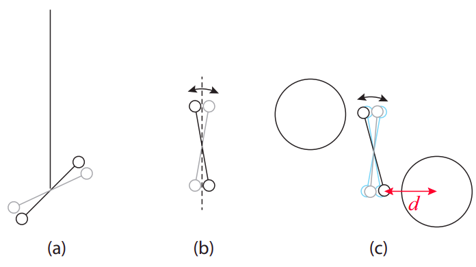
You have now made a torsion balance similar to the one Cavendish used. You will probably find out that it it is very hard to keep it motionless: the slightest displacement causes it to oscillate around an equilibrium position. The way it works is that an angular displacement \(\theta\) from equilibrium puts a small twist on the line, which results in a restoring torque \(\tau = −\kappa \theta\), where \(\kappa\) is the torsion constant for your setup. If your dumbbell has moment of inertia \(I\), then the equation of motion \(\tau = I \alpha\) gives you

\[I \frac{d^{2} \theta}{d t^{2}}=-\kappa \theta \label{eq:11.35} .\]

If you compare this to Equation (23.3.3), and follow the derivation there, you can see that the period of oscillation is

\[ T=2 \pi \sqrt{\frac{I}{\kappa}} \label{eq:11.36} \]

so if you measure \(T\) you can get \(\kappa\), since \(I = 2m(l/2)^2 = ml^2/2\) for the dumbbell.

Now suppose you bring two large masses, a distance \(d\) each from each end of the dumbbell, perpendicular to the dumbbell axis, and one on either side, as in the figure. The gravitational force \(F^G = GmM/d^2\) between the large and small mass results in a net “external” torque of magnitude

\[ \tau_{e x t}=2 F^{G} \times \frac{l}{2}=F^{G} l \label{eq:11.37} .\]

This torque will cause a very small displacement, so small that the change in \(d\) will be practically negligible, so you can treat \(F^G\), and hence \(\tau_{ext}\), as a constant. Then the situation is analogous to that of an oscillator subjected to a constant external force (section 23.2): the frequency of the oscillations will not change, but the equilibrium position will. In Equation (23.2.14) we found that \(y_{0}^{\prime}-y_{0}=F_{e x t} / k\) for a spring of spring constant \(k\), where \(y_0\) was the old and \(y_{0}^{\prime}\) the new equilibrium position (the force was equal to \(−mg\); the displacement of the equilibrium position will be in the direction of the force). For the torsion balance, the equivalent result is

\[ \theta_{0}^{\prime}-\theta_{0}=\frac{\tau_{e x t}}{\kappa}=\frac{F^{G} l}{\kappa} \label{eq:11.38} .\]

So, if you measure the angular displacement of the equilibrium position, you can get \(F^G\). This displacement is going to be very small, but you can try to monitor the position of the dumbbell by, for instance, reflecting a laser from it (or, one or both of your small masses could be a small laser). Tracking the oscillations of the point of laser light on the wall, you might be able to detect the very small shift predicted by Equation (\ref{eq:11.38}).

Historically, this experimental set up was used in the first precision calculation of the gravitational constant G, from the force \(F^G\). This experiment was carried out in the late 1790s by Henry Cavendish, but several others were involved in the several decades beforehand (you can check the story out on Wikipedia).