
7.4: Designing Molecular Membranes Models with VMD
- Page ID
- 17562
Introduction
While modern experimental techniques are able to resolve membrane-bound protein function, structural determination is still a challenge. To provide insight into the behavior of membranes and the proteins residing within them, computational biologists utilize molecular dynamics (MD) simulations. Since the early 2000’s there has been a remarkable increase in the number of computational methods, software, and visualization aids, reinforcing the need for MD [Ref. 1]. This tutorial is for users to become familiar with producing and visualizing atomistic membranes for MD simulations. This tutorial will use Visual Molecular Dynamics (VMD), a molecular visualization program of large biomolecular systems, to visualize membrane models. Additionally, the tutorial will discuss how CHARMM-GUI, a molecular systems generation web interface, can be used to build membrane models. Completion of this tutorial will allow the user to:
- Design, visualize, and select certain lipid sections using the VMD command interface.
- Visualize homogenous phosphatidylethanolamine ( POPE) and phosphatidylcholine (POPC) membranes using VMD’s MembraneBuilder extension tool.
- Create solvated, heterogenous lipid membrane models using the CHARMM-GUI Membrane Builder extension tool.
This tutorial uses a Linux 64 version of VMD (ver. 1.9.3 OpenGL). Other system downloads can be found here: www.ks.uiuc.edu/Development/Download/download.cgi?PackageName=VMD [Ref. 2]. Other versions may result in an inexact rendition of the tutorial, however, the concepts remain valid and should be practiced. Experimentation is encouraged. The CHARMM-GUI Membrane Builder extension can be found here: http://www.charmm-gui.org/?doc=input/membrane.bilayer [Ref. 3-8].
Note: text in italics indicates verbatim text/tools/commands that can be found/typed on your screen when going through the tutorials. User exercises are also indicated in italics. Figure references are highlighted in bold to indicate helpful visuals.
1. Basic VMD visualization of POPE
The Protein Data Bank (PDB) is the largest online repository containing more than 150,000 three-dimensional biological structures to date [Ref. 9-11]. Computational biologists frequently use the PDB as a starting point for their molecular models, either implementing existing PDB structures (as .pdb file formats) or formatting their own PDB template for molecular dynamics (MD). However, most PDB files do not contain membrane structure components; computational biologists typically design their own membranes and insert protein structures within them. Thus, this section is an introduction for new users on how to navigate Visual Molecular Dynamics (VMD) software before building membranes. This section will use the lipid phosphatidylethanolamine (POPE) as the example structure. For a review on lipid types and their properties, visit the BPH 241 Lipids webpage: https://phys.libretexts.org/Courses/University_of_California_Davis/UCD%3A_Biophysics_241_-_Membrane_Biology/Lipids
1.1. Contents of a .pdb file and loading the POPE model
Phosphatidylethanolamine ( POPE) is a glycerophospholipid and one of the most abundant lipid types in bacteria. In the downloadable files section (bottom of page), you will find the file 1.1_single_POPE.pdb. A .pdb file is a Protein Data Bank file containing all of the experimental and three-dimensional coordinate information needed to visualize the biomolecule (Figure 1.1). More information on .pdb files and their syntax can be found here: http://www.wwpdb.org/documentation/file-format [Ref. 12-13].

After downloading the VMD software, redirect to the VMD folder and open the README file for installation instructions. In addition to installation, Linux users will have to add a VMD path to their .bashrc file to call from the terminal. On the last line of your .bashrc file, add export PATH=/type/your/directory/here/vmd:$PATH (Figure 1.2). Now, the keyword vmd can be typed in the Linux terminal to launch VMD. Note: Some Linux distributions, Windows, and Mac devices as well as VMD software distributions may differ; always read the README file for the best installation guidance.

After launching VMD, you will see two windows: the VMD Main and the VMD Display. The VMD Main window contains the executable commands and options to manipulate the molecule on the VMD Display. Next, from the VMD main window, load the single_POPE.pdb file using File → New Molecule... A new window called the Molecule File Browser will appear. From here, click Browse and navigate to the folder containing single_POPE.pdb. After selecting, click Load in the Molecule File Browser window to load the POPE molecule to the VMD Display (Figure 1.3).
To create a new session, click File → New Molecule... 2) In the Molecule File Browser, files can be selected with the Browse button.
Once a file is selected the Molecule File Browser will determine the file type. A file is loaded by clicking the Load button.
3) Once a file is loaded, it will appear in the VMD Display window. In this example, a single POPE molecule is displayed as lines.
1.2 Basic VMD visualization features: orientation, rotation, and representation
The VMD Display has two primary mouse manipulation modes: rotate (press r on keyboard) and translate (press t on keyboard). More mouse mode commands can be found here: www.ks.uiuc.edu/Research/vmd/vmd-1.9.3/ug/node32.html [Ref. 14-15].
For rotate mode, the following mouse commands are:
- Left click and hold = free three-dimensional rotation
- Right click hold = rotation parallel to computer screen
- Mouse wheel = zoom in/out of center
For translate mode, the following mouse commands are:
- Left click and hold = translate molecule parallel to computer screen
- Right click and hold mouse wheel = zoom in/out of center
On the VMD Display, you should see the Lines representation of a POPE molecule; Lines representation is when atom types are represented by colored lines indicating the element type. In this model, the colors for each element are:
- cyan = carbon
- white = hydrogen
- red = oxygen
- orange = phosphorous
- blue = nitrogen
The Lines representation is helpful to visualize the entire molecule, but there are other representations that can be used. From the VMD Main, go to Graphic → Representations… A new window called Graphical Representations will appear (Figure 1.4). Here you will see a selected molecule tab where you can visualize different molecules. You will also see Draw style, Selections, Trajectory, and Periodic tabs that tweak the visual representation of each molecule.

Focus on the Draw style tab. In it, you can change the Coloring Method, the Drawing Method, the Material shading, and the Thickness of representation. Change the Thickness of the line from 1 to 5. It should be easier now to visualize the molecule. Reset the Thickness to 1.
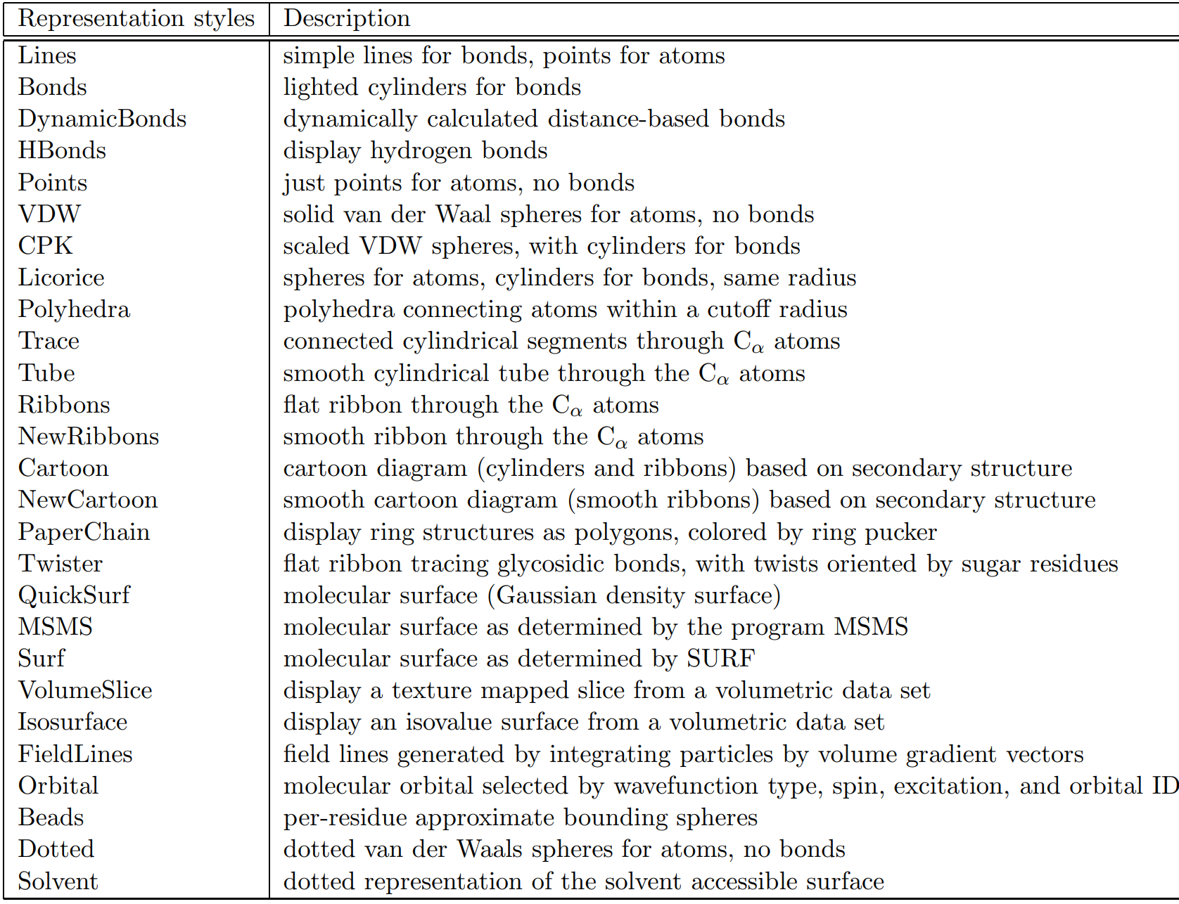
In the Drawing Method selection pane you will find different molecule visualization schema. Some common styles are Lines, VDW, and CPK (Figure 1.5), however there are other styles available (Table 1.1). The Lines style is the oldest style which uses lines as bonds and points as atoms. The VDW is a Van der Waals style and is a helpful space-filling representation. The CPK style can be thought of as a combination of Lines and VDW by providing scaled atoms as spheres linked by cylindrical bonds.
In the Coloring Method selection pane you will find different coloring schemes depending on atom typing, molecule collection, residue ID, and some physical properties. The effectiveness of these schemes will be dependent on your .pdb file parameters. For now, the single_POPE.pdb file is only useful with the Name method. Experiment with the various drawing/coloring methods. Afterwards, reset the molecule with Coloring Method: Name and Drawing Method: CPK.

The Lines style is useful for understanding structure, the VDW style for space-filling, and the CPK style as a mixed
style utilizing both Lines structure and CPK space-filling.
Table 1.1. Molecular draw styles from VMD User's Guide Version 1.9.3 [Ref. 15]
1.3. Identification of atom types
To label specific atoms, go to the VMD Main window and select Mouse → Label → Atoms. Clicking on an atom will show the molecule name followed by the atom name. From the color scheme, label the phosphorous atom followed by the nitrogen. To manage the labels, go to the VMD Main window and select Graphics → Labels… Here you can find a collection of the labels you have made. You can click on each label and show, hide, delete, and reposition them in the VMD Display (Figure 1.6). For example, select the POPE1:P (the phosphorous) atom label. Under the Picked Atom tab you will find the naming information (ResName, ResID, etc). In the Properties tab you can drag the crosshair in the Offset chart to reorient the label. In the Global Properties tab you can adjust your text size and thickness.
In addition to visualizing atom labels, you can visualize bond lengths and angles. Again, from the VMD Main window, select Mouse → Label → Bonds. To visualize a bond length or distance between atoms, you must click on the two atoms you are interested in measuring from. You can find the labeled distances from Graphics → Label in the VMD Main window. Similarly, you can calculate angles by clicking on three atoms (Figure 1.7). It is important to note that VMD cannot display double bonds since the .pdb file does not contain bond information. Indeed, PDB files contain coordinate information only. VMD compensates for this by using a distance measure algorithm to determine which atoms are bonded. Protein Structure Files can also be used to explicitly state bonding information but are beyond the scope of this tutorial. Therefore, an intuitive understanding is sometimes needed for the viewer to fully understand the model.

2) The atom distance between two hydrogen atoms as 2.03 Angstroms.
3) The angle between a carbon atom and two of its hydrogen bonding partners as 105.48 degrees.
Exercises (section 1.3)
Exercise 1.1: Identify one atom of each element: Carbon, hydrogen, oxygen, nitrogen, and phosphorous. Rearrange each label so that they are all visible while clearly indicating the atom.
Exercise 1.2: How many double bonds are there in POPE? Where would you expect double bonds?
1.4. Advanced selection of specific regions
As you create more complex models you’ll want to be able to specify a viewing region. This can be done by using the Graphical Representations window (Figure 1.4). Again, from the VMD Main, select Graphics → Representations… to open the Graphical Representations window. First, create a new representation of the selected molecule by clicking Create Rep. In the representation box you’ll now see two representations. By double-clicking you can hide the representation; hidden representations are in red text while visible representations in black text. Highlight the visible representation to enable it for editing.
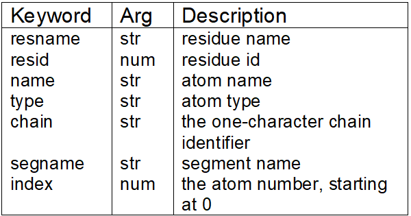
In the selected atoms box, you can utilize certain keywords to enable or disable parts of your model. You can even use more complex strings as well as boolean or numeric values to specify your selection criteria; VMD's expression system is based on PERL (a computing language) syntax. Examples of these regular expressions can be found in section 6.3 of the VMD User's Guide [Ref. 15]. Back in the Labels window (Graphics → Label) you may have noticed certain labels having type information in the Picked Atom tab (Figure 1.6). Keywords such as ResName, ResID, Name, Type, Chain, SegName, and Index can be used to specify a selection (Table 1.2); descriptions of all keywords can be found in section 5.48 of the VMD User's Guide [Ref. 15]. For now, since there is only one POPE molecule labeled as ResName: POPE and specified as Chain: X, sort through the atom types for practice. To visualize all carbon atoms, use a regular expression such as (Figure 1.8):
- name “C.*”
where the C represents the canonical carbon atom naming convention and the .* indicates any carbon atoms in the model. In an expression, this example means to search for anything classified as a name that starts with C. Another way to visualize carbon only atoms is by typing:
- not name “O.*” and not name “P.*” and not name “H.*” and not name “N.*”
Your representation should not have changed as you’ll only see carbon atom types. In more complex models, you can specify single molecule chains or even molecule types:
- resname POPE
- chain X
In both of these cases you should see the entire phosphatidylethanolamine ( POPE) molecule. More selection expressions can be found in Chapter 6.3 of the VMD 1.9.3 User's Guide [Ref. 15]
Table 1.2. Examples of commonly found keywords for selection of specific model
regions. Argument identifiers are: str=string and num=number. More information
on other keywords can be found in [Ref. 15].
Exercises (section 1.4)
Exercise 1.3. Visualize all atoms but carbon in the single_POPE.pdb file.
Exercise 1.4. Using the index notation, visualize the polar head group. Hint: index notation for VMD starts at zero.
1.5 Saving and loading your session
From VMD Main, select File → Save Visualization State… Here you can specify which folder and what file name you would like using traditional file path syntax: user/home/my_folder/my_file_name.vmd Make sure you save as a .vmd or you will be unable to load the file! If you forget, rename your file so that you include the .vmd file type. To load your session, start VMD and from VMD Main select File → Load Visualization State… Note: File → New Molecule… is for importing new molecule file types only. It is better to use the Load Visualization State if you want to preserve your model representation settings (Figure 1.9).

2. Homogenous membranes using VMD’s MembraneBuilder tool
The purpose of the Visual Molecular Dynamics (VMD) MembraneBuilder tool is to generate a membrane model surrounded by water which a protein can then be placed into. This complete lipid/protein/water model can then be used to run molecular dynamics simulations after generation of force field components and simulation parameters; a review on force fields can be found at [Ref. 16]. For this tutorial, the MembraneBuilder tool extends our interpretation of individual phosphatidylethanolamine ( POPE) molecules to a homogenous POPE membrane. Unfortunately, the MembraneBuilder tool can 1) only generate homogenous POPE and phosphatidylcholine (POPC) membranes and 2) generate only water surrounding molecules. For more information on how MembraneBuilder executes its algorithm, visit here: www.ks.uiuc.edu/Research/vmd/plugins/membrane/ [Ref. 17]. For homogenous or heterogeneous membranes with the option of ion solvation, skip this section and proceed to Section 3 which uses the CHARMM-GUI interface to generate membranes.
2.1 Generate a POPE membrane
From VMD Main, select Extensions → Modeling → Membrane Builder to open the Membrane window. In this window, select phosphatidylethanolamine (POPE) as the lipid, and generate a 50x50 Angstrom2 area. Change the output prefix to POPE_membrane. The topology section provides two CHARMM force fields that can be used: CHARMM27 and CHARMM36. Generally, CHARMM27 is for nucleic acids and lipids while CHARMM36 is for proteins and lipids; CHARMM36 is noted to have superior lipid parameters and thus should be used for most membrane biology models [Ref. 18]. After selecting CHARMM36 (c36), click Generate Membrane. You should now see a POPE membrane that is 50x50 Angstrom2 with the leaflets surrounded by water. You will also note some patterns of randomness and discontinuity; perfect membranes are physiologically impossible thus stochasticity (randomness) is modeled. Visualize the membrane using a CPK Drawing Method as described in Section 1.2 (Figure 2.1).
window allows users to generate a specific area (in Angstroms) of membrane. The membrane options are POPE and POPC with generation force fields
using either CHARMM27 (c27) or CHARMM36 (c36) 3) A side view of the generated POPE membrane with surrounding water from the tutorial instructions.
Next, verify the generated membrane x-y length. From the Graphical Representations window (Figure 1.4), remove the water by typing in the Selected Atoms text box:
- not water
In the VMD Main, select Mouse → Label → bonds. Using the x-, y-, and z-planes, take 5 rough measurements and record the average; a review on how to do this is in Section 1.3. You’ll notice that the membrane area will be less than 50 Angstrom2 (around 45 Angstrom2 average). This is likely due to the close packing arrangement performed after initial generation of the model. You can save these models as discussed in Section 1.5 or save the membrane as a PDB coordinate file. From the VMD Main, File → Save Coordinates… will open a Save Trajectory window where you can select the molecule, atoms, and file format you wish to save as.
Exercises (section 2.1)
Exercise 2.1. Take an average of 5 measurements to determine the thickness of the membrane bilayer. Does this match experimental values? Section 1.3 describes how to measure distances.
Exercise 2.2. Take an average of 5 measurements to determine the water thickness. Why does the model need water? Should thickness be lower? Should thickness be higher?
3. Heterogeneous membrane building using CHARMM-GUI Membrane Builder
The CHARRM (Chemistry at HARvard Macromolecular Mechanics) force field was initially developed for proteins and nucleic acids but has since been extended to feature a robust set of lipid types [Ref. 19-20]. The most recent force field, CHARMM36, supports proteins, nucleic acids, carbohydrates, lipids, and small molecules [Ref. 21]. CHARMM-GUI is an online graphical user interface that allows the generation of multiple MD models and preliminary input files for the start of simulation [Ref. 4-8]. This section will cover the Membrane Builder tool that allows users to develop membrane models with the option of including protein complexes. For this tutorial, only the bilayer builder section, without protein insertion, and without preliminary simulation building will be discussed. While there are other membrane building options, the bilayer builder is the simplest all-atom tool to work through for beginners. Alternatively, some membrane building tools do not utilize all-atom modeling; for an alternative atom modeling schema see Course Grained Simulations:
Note : should you want to try protein-membrane model building in the future, make sure your protein PDB has the correct orientation relative to the membrane or you will improperly insert your protein. Improper protein insertion will result in simulations not reflecting real-life predictions since the protein is not in a physiological state. A tutorial on protein insertion can be found here: www.ks.uiuc.edu/Training/Tutorials/science/membrane/mem-tutorial.pdf [Ref. 22].
3.1. Determine lipid components, size, and solvation
Click on the following link to reach the CHARMM-GUI Membrane Builder Bilayer Builder webpage: http://www.charmm-gui.org/?doc=input/membrane.bilayer [Ref. 3]. Scroll down to find a brief explanation of the workflow, an option to include a Protein Data Bank (.pdb) file, and an option to generate a membrane only system. Click the Membrane Only System to be redirected to the System Size Determination Options page (Figure 3.1).

1) An option to create a protein/membrane system with a .pdb is provided.
2) For this tutorial, select "Membrane Only System."
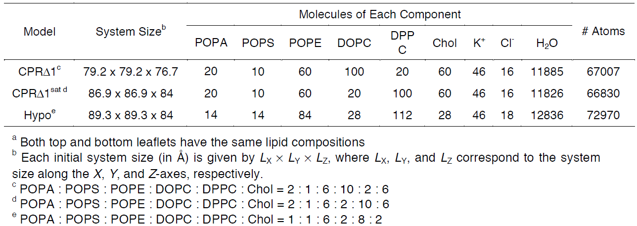
For this tutorial, users will recreate a model that has been used to study the effects of lipid tail saturation [Ref. 6]. The model is the CPRΔ1 model, a yeast-like model that contains a relatively high concentration of unsaturated lipids. In the System Size Determination Options, click the Heterogeneous Lipid, the Water thickness, and the Ratios of lipid components options. Next, input 20 Angstroms as the water thickness, and input 80 Angstroms as the initial X-Y guess (Figure 3.2). The initial X-Y guess is dependent upon the problem being solved; for example, a larger membrane protein would require a larger membrane area in order to be embedded. Below the system size is the lipid components options (Figure 3.3). Fill in the lipid ratios as indicated in Table 3.1. When finished, click the Show the System Info button and verify the generated dimensions. Ideally, both leaflets should have close to the same surface area; uneven areas can induce membrane bending artifacts during simulations and thus would be non-physiological. Once the system dimensions calculate near identical leaflet areas, click Next Step: Determine the System Size located in the lower right of the CHARMM-GUI webpage. This step may take some time. Do not close or refresh the CHARMM-GUI webpage.
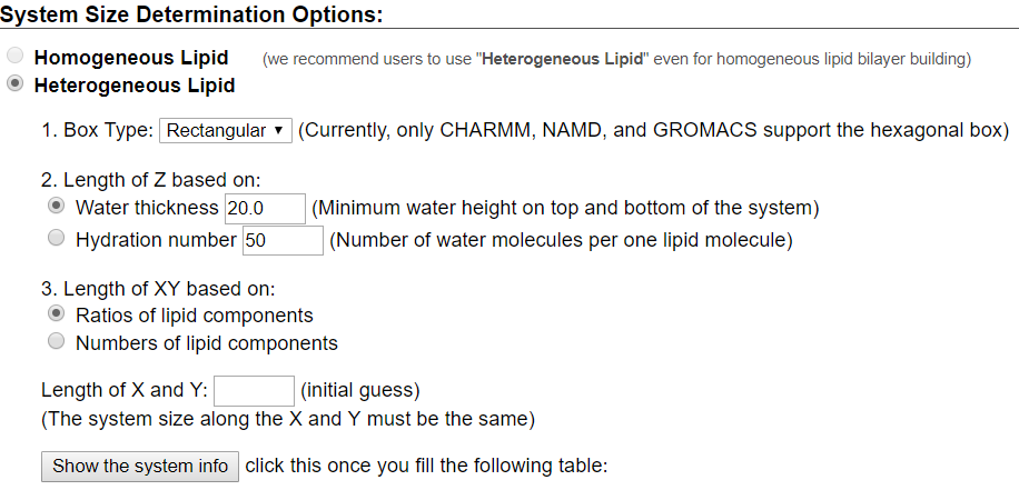
will vary depending on desired physiological parameter being studied,
desired computational processing speed, and MD software used.
For the tutorial, use 80 Angstroms as the initial X-Y guess.

Make sure you click "Show the system info" after you input your desired lipids
to verify near identical leaflet areas!
Table 3.1. Representative model components from supplemental Table 2 in So S. et al, 2009 [Ref. 6]. These lipid
components will be used for the tutorial section to demonstrate how CHARMM-GUI can be used to model biophysical problems.
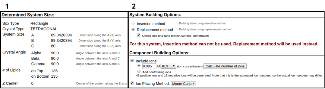
In the next web page, you will have a system output box showing you the various CHARMM parameter files generated from the previous step (Figure 3.4). You can download the system parameter files at any step during the tutorial by clicking download.tgz in the top right of the CHARMM-GUI webpage. You can view the Generated Packed System by clicking view structure; this will open an additional window that can be manipulated similar to the Visual Molecular Dynamics (VMD) display. Viewing the structure after each step is helpful in understanding how CHARMM-GUI constructs the model. In this step, only the packing arrangement has been determined (Figure 3.4). Below the system output box you will see the Determined System Size section with size parameters for building the system. Further down you will see the System Building Options section (Figure 3.5). A key component of system building is deciding if the insertion or replacement method of adding model components should be used. Generally, insertion methods are meant for protein insertions into bilayers while membrane-only models should use the replacement method. Additionally, enable the Check lipid ring penetration box to verify that lipid replacement does not produce positional artifacts. Next, in the Component Building Options section, ions are included in the system to generate a charge neutral model for electrostatic calculations during the simulation. For this case, we want to mimic the number of ions listed in Table 3.1. Adjust the ion concentration until you have exactly the correct number of ions. For this tutorial, use the Monte Carlo ion placement method (Figure 3.5). Once finished, click Next Step: Build Components located in the lower right of the CHARMM-GUI webpage. This step may take some time. Do not close or refresh the web page.
1) Click on the step3_packing.pdb (blue arrow) to view the structure. 2) A top-down view of the packing arrangement indicated as orange spheres.
The pink and blue squares indicate the upper and lower leaflet faces, respectively. This model view can be rotated similar to the VMD Display.
3.2. Final assembly, export, and visualization
Step 4 of the CHARMM-GUI Membrane Builder provides a self-check for lipid ring penetration as well as ion/water box building. In the system output box at the top of the page you can find the step4_lipid.pdb structure for viewing (Figure 3.6). Click Next Step: Assemble Components.
This model is the step before solvation.
Step 5 of the CHARMM-GUI Membrane Builder provides force field options, input generation options, and equilibration options for generating M.D. simulation parameters. Input options can be generated for various M.D. force fields such as GROMACS, AMBER, and CHARMM, among others. The use of a force field will largely be dependent upon your experimental question and your lab's computational expertise. A review describing the necessity for force fields and some common types can be found at [Ref. 16].
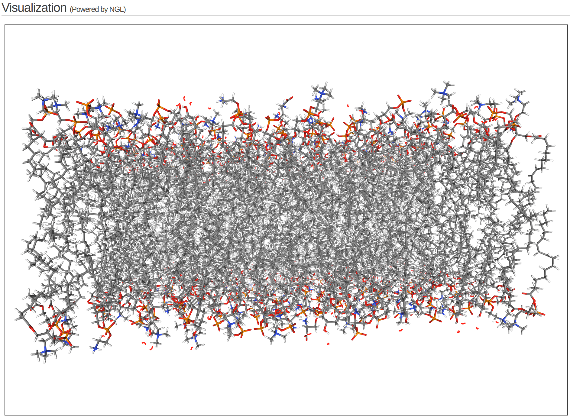
At the top of the system output box you will see the assembled .pdb file labeled as step5_assembly.pdb. You can download this .pdb file or the entire CHARMM-GUI folder by clicking the download.tgz icon at the top right of the CHARMM-GUI webpage. After downloading, the final model can be visualized using VMD as described in Section 1 (Figure 3.7).


(Right) side view of generated membrane model from tutorial.
Exercises (section 3.2)
Exercise 3.1. From the complete model (Figure 3.7), isolate each class of lipid, ion, and water atoms as their own representation. Hint: you may need to look at the .pdb file in a text editor or in the VMD Labels feature to find common naming schemes.
Exercise 3.2. Generate the other two models from Jo, S. et al 2009 (Table 3.1) [Ref. 6]. What do you expect will be different compared to the CPRΔ1 model?
Exercise 3.3. Find another biomembrane of interest and generate the model. What parameters must you know to ensure that it is physiologically relevant?
Exercise 3.4. Temperature can be a critical factor during M.D. system equilibration. As seen in CHARMM-GUI Membrane Builder step 5, there is an option to adjust the temperature. What are reasonable/unreasonable temperatures? What is a good rule of thumb? Hint: Membrane fluidity.
Exercise 3.5. Review the following article [Ref. 23] for examples on how molecular simulations have helped validate and promote experimental findings. What stood out to you? Which experiment did you find most interesting?
Acknowledgments
Some images were made with VMD/NAMD/BioCoRE/JMV/other software support. VMD/NAMD/BioCoRE/JMV/ is developed with NIH support by the Theoretical and Computational Biophysics group at the Beckman Institute, University of Illinois at Urbana-Champaign.
Some images were made with the online CHARMM-GUI visualization tool during Section 3: Heterogeneous membrane building using CHARMM-GUI Membrane Builder.
References
[1] Hospital, A., Goñi, J. R., Orozco, M., Gelpí, J. L. (2015). Molecular dynamics simulations: advances and applications. Adv Appl Bioinform Chem. 8(1): 37-47. doi: 10.2147/AABC.S70333
[2] Software downloads download VMD. Available at www.ks.uiuc.edu/Development/Download/download.cgi?PackageName=VMD
[3] CHARMM-GUI Membrane Builder. Available at http://www.charmm-gui.org/?doc=input/membrane.bilayer
[4] Jo, S., Kim, T., Iyer, V. G., Im, W. (2008). CHARMM-GUI: a web-based graphical user interface for CHARMM. J Comput Chem. 29(11): 1859-1865. doi: 10.1002/jcc.20945
[5] Wu, E. L., Cheng, X., Jo, S., Rui, H., Song, K. C., Dávila-Contreras, E. M., Qi, Y., Lee, J., Monje-Galvan, V., Venable, R. M., Klauda, J. B., Im, W. (2014). CHARMM-GUI Membrane Builder toward realistic biological membrane simulations. J Comput Chem. 35(27): 1997-2004. doi: 10.1002/jcc.23702
[6] Jo, S., Lim, J. B., Klauda, J. B., Im, W. (2009). CHARMM-GUI Membrane Builder for mixed bilayers and its application to yeast membranes. Biophys J. 97(1): 50-58. doi:10.1016/j.bpj.2009.04.013
[7] Jo, S., Kim, T., Im, W. (2007) Automated builder and database of protein/membrane complexes for molecular dynamics simulations. PLoS One 2(9): e880. doi: 10.1371/journal.pone.0000880
[8] Lee, J., Patel, D. S., Ståhle, J., Park, S. J., Kern, N. R., Kim, S., Lee, J., Cheng, X., Valvano, M. A., Holst, O., Knirel, Y. A., Qi, Y., Jo, S., Klauda, J. B., Widmalm, G., Im, W. (2019). CHARMM-GUI Membrane Builder for complex biological membrane simulations with glycolipids and lipoglycans. J Chem Theory Comput. 15(1): 775-786. doi: 10.1021/acs.jctc.8b01066
[9] PDB statistics: overall growth of released structures per year. (2019). Available at: www.rcsb.org/stats/growth/overall
[10] Berman, H. M., Westbrook, J., Feng, Z., Gilliland, G., Bhat, T. N., Weissig, H., Shindyalov, I. N., Bourne, P. E. (2000). The Protein Data Bank. Nucleic Acids Res. 28(1): 235-242. doi: 10.1093/nar/28.1.235
[11 ] Burley, S. K., Berman, H. M., Bhikadiya, C., Bi, C., Chen, L., Di Costanzo, L., Christie, C., Dalenberg, K., Duarte, J. M., Dutta, S., Feng, Z., Ghosh, S., Goodsell, D. S., Green, R. K., Guranovic, V., Guzenko, D., Hudson, B. P., Kalro, T., Liang, Y., Lowe, R., Namkoong, H., Peisach, E., Periskova, I., Prlic, A., Randle, C., Rose, A., Rose, P., Sala, R., Sekharan, M., Shao, C., Tan, L., Tao, Y. P., Valasatava, Y., Voigt, M., Westbrook, J., Woo, J., Yang, H., Young, J., Zhuravleva, M., Zardecki, C. (2019). RCSB Protein Data Bank: biological macromolecular structures enabling research and education in fundamental biology, biomedicine, biotechnology and energy. Nucleic Acids Res. 47(D1): D464-D474. doi: 10.1093/nar/gky1004
[12] PDB file format documentation. Available at: http://www.wwpdb.org/documentation/file-format
[13] Berman, H., Henrick, K., Nakamura, H. (2003). Announcing the worldwide Protein Data Bank. Nat Struct Biol. 10(12): 980. doi: 10.1038/nsb1203-980
[14] Mouse modes. (2019). Available at: www.ks.uiuc.edu/Research/vmd/vmd-1.9.3/ug/node32.html
[15] VMD user's guide version 1.9.3. (2016). Available at www.ks.uiuc.edu/Research/vmd/vmd-1.9.3/ug.pdf
[16] González, M. A. (2011) Force fields and molecular dynamics simulations. Collection SFN 12(1): 169-200. doi: 10.1051/sfn/201112009
[17] Balabin, I. Membrane plugin, version 1.1. Available at www.ks.uiuc.edu/Research/vmd/plugins/membrane/
[18] Huang, J., MacKerell, A. D. Jr. (2013) CHARMM36 all-atom additive protein force field: validation based on comparison to NMR data. J Comput Chem. 34(25): 2135-2145. doi: 10.1002/jcc.23354
[19] Brooks, B. R., Bruccoleri, R. E., Olafson, B. D., States, D. J., Swaminathan, S., Karplus, M., (1983). CHARMM: A program for macromolecular energy, minimization, and dynamics calculations. J Comput Chem. 4(2) 187-217. doi: 10.1002/jcc.540040211
[20] Brooks, B. R., Brooks III, C. L., MacKerell Jr., A. D., Nilsson, L., Petrella, R. J., Roux, B., Won, Y., Archontis, G., Bartels, C., Boresch, S., Caflisch, A., Caves, L., Cui, Q., Dinner, A. R., Feig, M., Fischer, S., Gao, J., Hodoscek, M., Im, W., Kuczera, K., Lazaridis, T., Ma, J., Ovchinnikov, V., Paci, E., Pastor, R. W., Post, C. B., Pu, J. Z., Schaefer, M., Tidor, B., Venable, R. M., Woodcock, H. L., Wu, X., Yang, W., York, D. M., Karplus, M. (2010). CHARMM: the biomolecular simulation program. J Comput Chem. 30(10): 1545-1614. doi: 10.1002/jcc.21287
[21] Kessel, A. and Ben-Tal, N. (2018) Introduction to proteins structure, function, and motion second edition. Boca Raton, FL: CRC Press, Taylor & Francis Group.
[22] Aksimentiev, A. Sotomayor, M., Wells, D., Mahinthichaichan, P. (2016) Membrane Proteins Tutorial. Available at http://www.ks.uiuc.edu/Training/Tutorials/science/membrane/mem-tutorial.pdf
[23] Hollingsworth S. A., Dror, R. O. (2018) Molecular dynamics simulation for all. Neuron 99(6): 1129-1143. doi: 10.1016/j.neuron.2018.08.011