1.4: Working With the Energy-Interaction Model

Energy-Interaction Diagrams

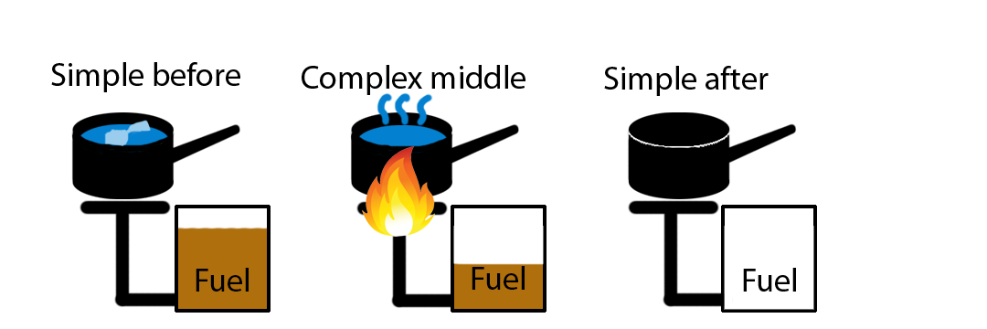
When solving complex energy interaction problems, it is often helpful to use a tool that was developed for this course, the Energy-Interaction Diagram. Energy-Interaction diagrams illustrate the types of energy transformations that occur when an open physical system is interacting with its environment, or with two or more substances which defined a closed physical system interact with each other. The diagram helps make clear the physical systems involved, the particular types of energy involved, and the changes in those energies resulting from the interaction over a given time interval. The initial and final states of the systems should be clearly indicated on the diagram. These diagrams are “before-to-after” diagrams. That is, they indicate the state of the systems before the interaction occurs and the state of the systems after the interaction has occurred, while not specifying any details of how the system got from the initial to the final state. We use Energy-Interaction diagrams because they are useful. They help us to systematically apply the energy conservation approach to a particular physical situation using the Energy-Interaction Model.

Figure 1.3.1: Illustration of the "before" and "after".

 

Drawing Energy-Interaction Diagrams When Modeling an Interaction in a CLOSED System:

1. The beginning and ending of the interaction is specified by explicitly writing down a condition of the physical system that corresponds to the beginning and end of the time interval over which the interaction occurs. These times are referred to as the initial and final times.
2. The types of energy that changed during the specified time interval are indicated by circles and labeled sufficiently to identify the type of energy.
3. If transfers of energy to the environment are significant, due to friction, for example, include the thermal system of the environment on the Energy-Interaction diagram. That is, enlarge the boundary of the closed system to include the environment.
4. The change in each energy, whether an increase or decrease, is indicated, when known, with an “up” or “down” arrow.
5. Changes in the observable parameter (indicator) associated with each type of energy that occur as a result of the interaction should be shown. If the quantitative change in the value is known, it should be given. If not, an “up” or “down” arrow can be used following the symbol of the indicator to indicate an expected increase or decrease.
6. Draw a solid oval around all the "energy circles" to indicate the system is closed.
7. Below the diagram write the energy-conservation equation. You may also indicate which quantities are positive or negative for each term in the equation.

Drawing Energy-Interaction diagram Diagrams When Modeling an Interaction in an OPEN System:

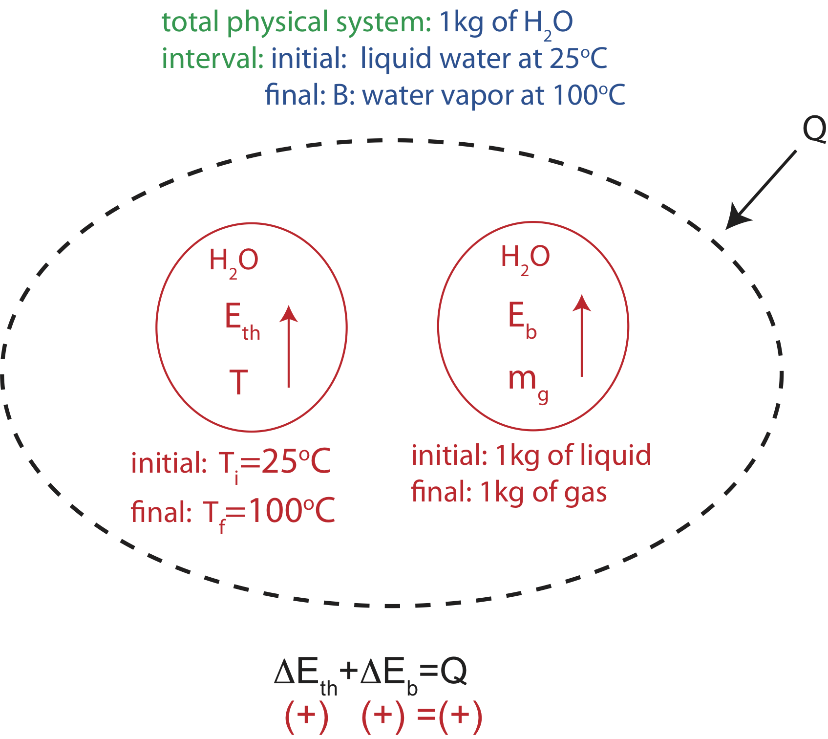
The important difference between open and closed systems is that energy from outside the open physical system can be transferred into or out of the physical system as heat, Q, or work, W. (By definition, these transfers do not occur for a closed system.) The only difference, then, in the Energy-Interaction diagram for the two types, is that the diagram for an open system needs to explicitly show the transfer of Q and/or W. This is done by drawing a dashed oval around all of the energies (to indicate the open physical system boundary) and drawing arrows pointing toward or away on the boundary to show a Q or a W transfer in or our, respectively. A generic example of the Energy-Interaction Diagram for an open system is shown below.

Figure 1.3.2: Generic Example of an Energy-Interaction Diagram in an open physical system with two substances, three types of energy, and heat leaving the system.

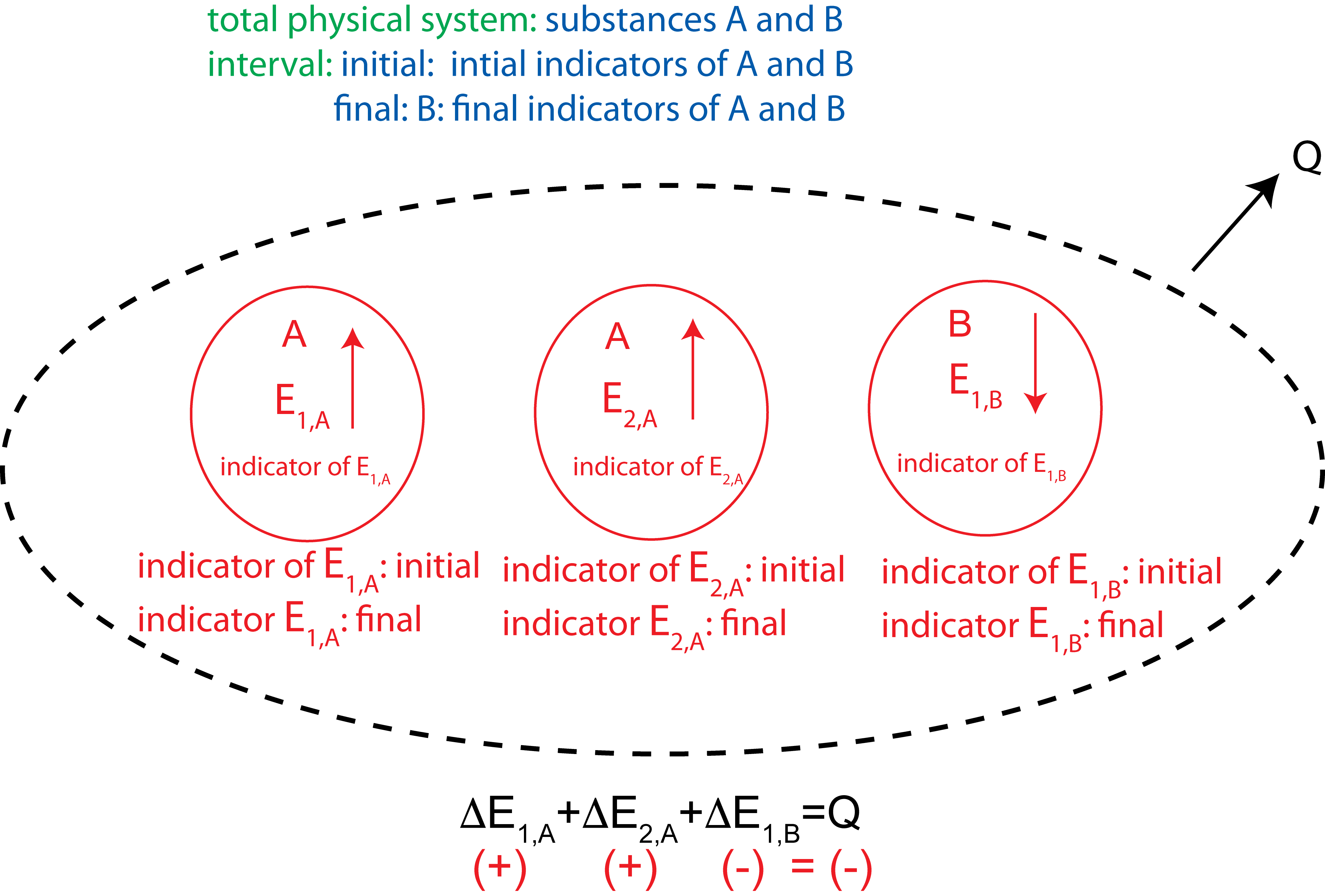
Comments:

1. What is shown in the diagram above is the minimum that must always be written down. Most of the hard thinking will have been done to get to this point. Often, many explanations of physical phenomena can be constructed using this diagram without going further and substituting in explicit expressions for the individual change in energy terms and numerical values for various parameters. Even if you are required to continue the process through to a numerical result, you must do the mental work of constructing the Energy-Interaction Diagram to this point prior to doing any numerical calculations.
2. In an open-system diagram, the arrow showing energy transfer into the system is drawn in the direction of energy flow and labeled with Q or W. Do not write "-Q" or "-W" when energy is transferred out of the system. The arrow pointing away from the system is the indication that Q or W is a negative quantity. The variable itself is a quantity that could be either positive or negative. The sign is added when the variable is converted to a numerical value.

General Process of Constructing an Energy-Interaction Diagram

Listed here are some general questions you need to ask yourself as you use the Energy-Interaction Model. The order suggested is logical, but it is often necessary to cycle back to previous questions depending what is known about the interaction. The Energy-Interaction diagram is a tool to help you use the Energy-Interaction Model, which helps you keep track of the many important details you need as you construct the model corresponding to the particular physical situation you are interested in.

Here is a list of common questions:

1. What happened? State the essence of the physical phenomenon of interest in your own words. You do not need to write this down, but you should have an “internal dialogue” with yourself.
2. What is the boundary of the physical system you are modeling? Answer this question by listing the physical things you intend to include in the physical system. (Examples of “physical things” are: air, H₂O, your hand, heat pack, all of the chemicals.)
3. What is the extent of the process or interaction? This means identifying the beginning and end of the time interval corresponding to the process/interaction that you defined and explicitly writing this on the diagram.
4. Which energy types do you include in your diagram? Answer: Which indicators are changing? Each indicator that changes corresponds to a type of energy that changes. Put these energies into your diagram as labeled circles (for example, “H₂O E_thermal”). Include the indicator for each type of energy inside the labeled circle with an up or down arrow showing whether the indicator increased or decreased during the process, if known.
5. What are the values of the indicators at the times corresponding to the start and end of the interval you chose in step (3)? Record the initial and final values of the indicators next to their respective energies. Remember that all of the initial and final values of indicators should correspond to the same initial and final times. Note: It is not always necessary to identify specific initial and final values for all indicators. Sometimes, depending on the question, you only care about the change in the indicator (e.g., \(\Delta T\)). At other times, you may only know that the final value of the indicator is greater than (or less than, or equal to) the initial value. The point is not to memorize a series of steps, but to be as specific as possible about what you know. The diagram is not an end in itself, but a tool to lead you through your analysis and help you organize your thoughts. The diagram helps you connect the particular physical phenomenon to the particular model you are constructing.
6. Is the physical system in your particular model open or closed? If you are modeling the phenomenon as an open physical system, draw a dashed oval enclosing all of the energies, and use an arrow that stops or starts on the oval to show heat or work entering or leaving the physical system. You may find it necessary to go back to step (2) and modify the boundary of the physical system.
7. Write an equation expressing energy conservation for your particular Energy-Interaction diagram, in terms of the \(\Delta Es\), \(Q\), and/or \(W\). Each term in your conservation of energy equation must correspond to an "energy circle" in your diagram. Note, the main purpose of drawing the Energy-Interaction diagram is to help you write down the energy-conservation equation. If you get very comfortable with this model, you can go directly to this step and skip drawing the diagram, unless you are explicitly asked to do so.

Of course, much more complicated paths than following steps 1)-7) are possible. The following example illustrates how this is handled.

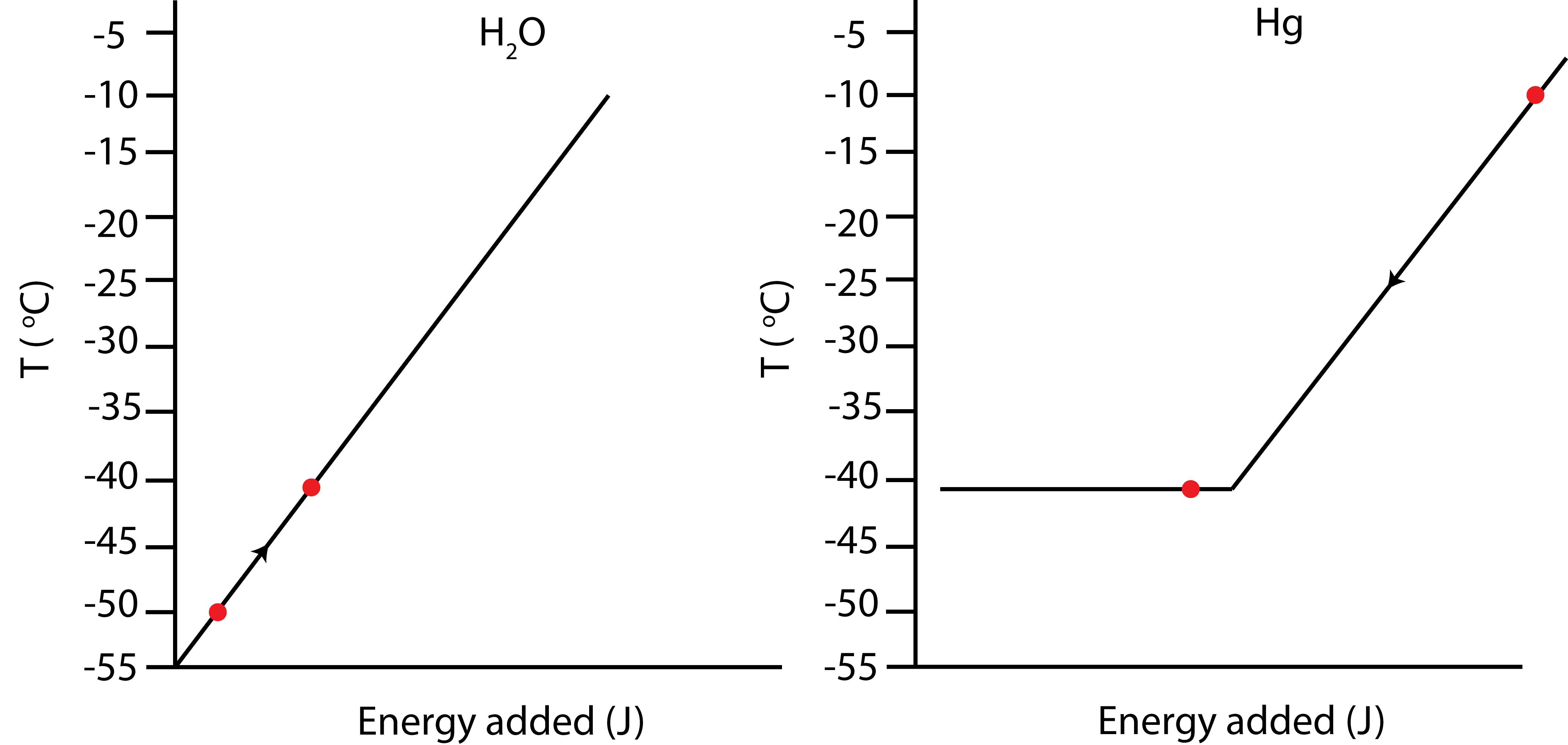
Example \(\PageIndex{1}\)

Depicted below are temperature vs. energy added plots for substances A and B. Substance A is initially at -5°C. Substance B is initially in the gas phase at its boiling temperature of 10°C. Assume all phases exist for both substances. When the two substances are brought into contact, they eventually reach thermal equilibrium. During this process 30 joules are released to the environment.

a) Label on the above plot the initial and final states for both substances.

b) Depict this process using an Energy-Interaction diagram.

 

Solution

a) Substance B is initially at a higher temperature than A, thus it will be losing energy and A will be gaining energy. Energy conservation tells us that the energy gained by A plus the energy lost by B have to equal to the energy released to the environment:

\[ \Delta E_{tot}(A)+\Delta E_{tot}(B)=Q=-30J \nonumber\]

Thus, B will loose 30 more joules than A will gain.

Starting points, which are stated in the problem, are marked on the plot below. Let us assume B will condense completely to liquid. This will result is a loss of 60J for B, thus a gain of 30J for A. If A gains 30J its temperature will be 5°C, B is at 10°C, so equilibrium is not yet achieved. For B to go to 5°C requires \(\Delta E_{tot}(B)=-70J\). This means \(\Delta E_{tot}(A)=40J\), where A is still at 5°C exactly half melted as shown by the “final” dot on the plot.

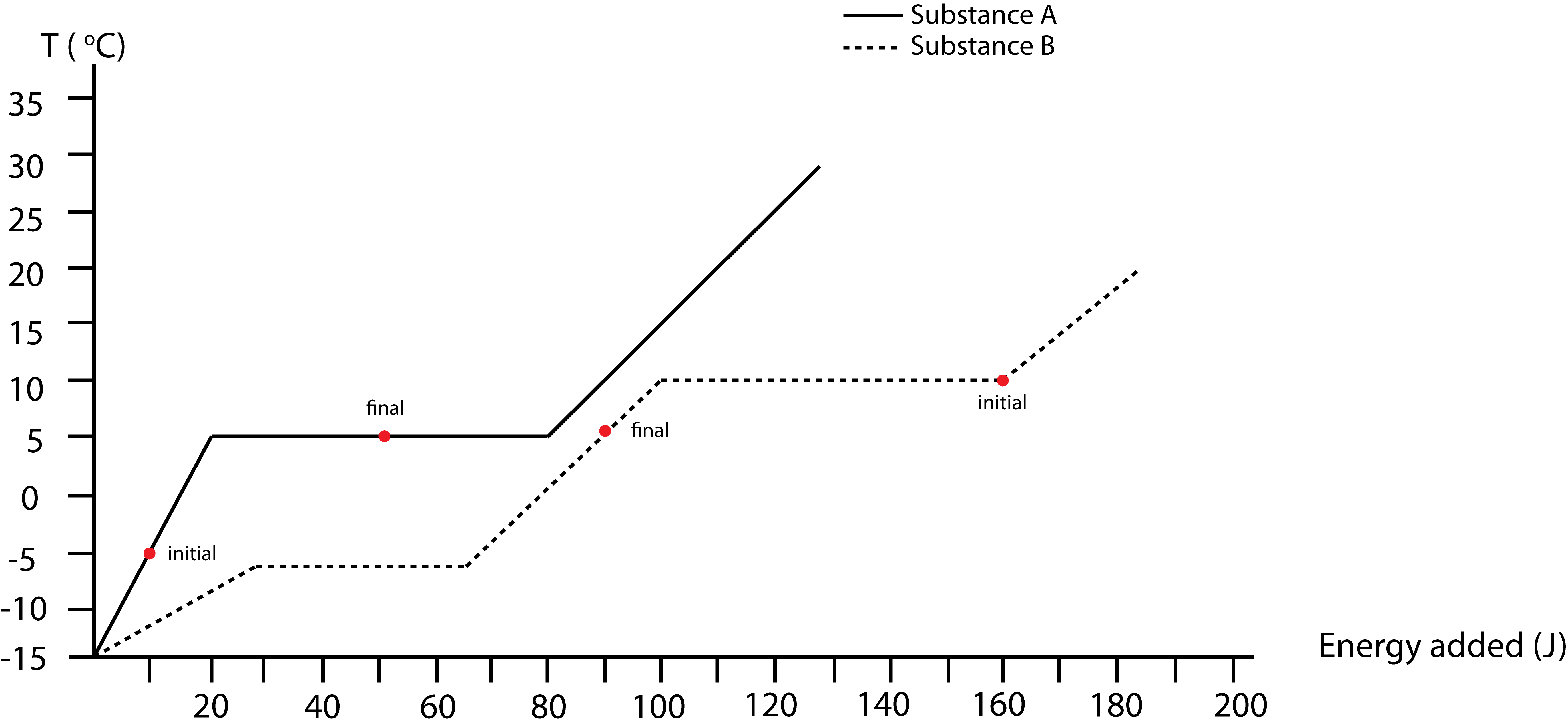
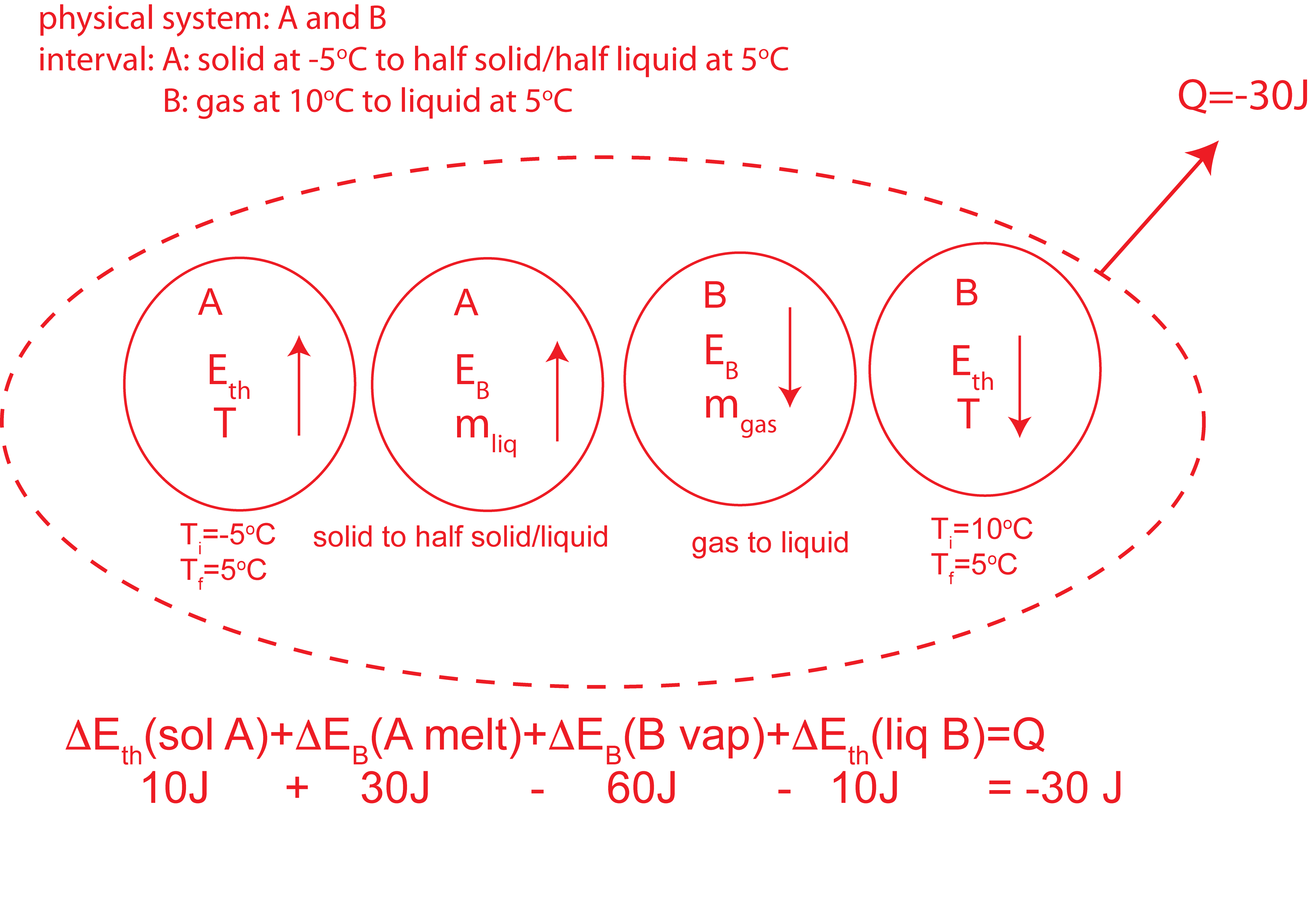
b) Based on the initial and final states, A will go through a thermal energy change in the solid phase and bond energy change from all solid to half solid/liquid. B will go through a bond energy change all gas to all liquid, and a thermal energy change in the liquid phase. The Energy-Interaction Diagram for this process is shown below.

 

Boiling a Pot of Water

Let us consider the physical situation of a pot of water left on an unattended kitchen stove top. We might wish to estimate how long it would take for 1.0 liter (1.0 kg) of water in the pan to boil away and heat the pan to dangerously high temperatures, perhaps igniting the plastic handle. Let us also suppose we have previously determined the rate at which energy is transferred from the stove burner to the pan by doing a simple experiment to see how long it takes to heat the 1 kg of water in the pan by 10°C, giving a calculated power input to the water of 1.0 kW. Power is a useful measure of energy transfer, since it tells us how fast energy is transferred, or the rate of energy transfer. Thus, power has units of energy per unit time. Watts is defined as \(W=J/sec\).

In this example we are both heating the water starting from room temperature of 25°C and changing its phase. Thus, we need to include both the thermal and bond energies of the water. Since we know there is a heat input to the pan of 1.0 kW, it makes sense here to model the water as an open system with the heat input from “the outside.” However, can we assume that all the energy is transferred to the water and neglect any transfer to the pan or the environment? If the mass of the water (1.0 kg) is several times larger than the mass of the pan (typically the case), the heat capacity of the pan will be considerably less than the water, since the specific heat of the water is so much greater than steel or aluminum and the amount is also larger in this case. The energy transfer to the environment from the pan is tougher to estimate. We do know from experience that water does boil when left on the burner for awhile. So the transfer to the environment is definitely less than from the stove to the pan. We can initially leave this out of the model, and consider whether to put it in when we have made the time calculation.

So at this point, our Energy-Interaction Diagram would look like this:

Figure 1.3.3: Energy-Interaction Diagram for boiling water

Plugging in the algebraic expressions for each kind of energy (Equations 1.3.4 and 1.3.6):

\[mc_{liq}\Delta T+m\Delta H_{vap}=Q \]

Looking up the values for water in Table 1.4.3, \(c_{liq}=4.18~kJ/Kkg\) and \(\Delta H_{vap}=2257~kJ/kg\) and plugging into the above equation:

\[(1kg)(4.18~kJ/Kkg)(75K)+(1kg)(2257~kJ/kg)=2571~kJ=Q \]

Since the heat input is 1 kW or 1 kJ/s, it would take about 2571 sec or 43 min to boil away the water.

Now let us examine whether our numerical predictions make sense. First, notice that the calculated change in bond energy is about seven times greater than the change in thermal energy. This is at least consistent with the values of heat capacities and heats of vaporization listed in the data table. (We will develop a much deeper understanding of this difference when we further develop our particle model of matter in Chapter 3.) This difference in heats also implies that the water would come to boiling much quicker than it would take to boil it away (about 5 minutes compared to 38 minutes). Does this correspond to your personal experience when cooking? Earlier, we raised the question whether the pan had an effect on the system. If we included the pan, which energies would we need to add? How would this affect our prediction of the time to boil away all of the water?

Example \(\PageIndex{2}\)

In an experiment 0.5kg of ice initially at -50°C is mixed some mercury initially at -10°C in an insulated container. Once the two substances come to thermal equilibrium 0.2 kg of mercury has frozen. Assume the total mass of Hg is bigger than 0.2kg. Use Table 1.4.3 to look up any relevant constants.

a) Depict the process using an Energy-Interaction diagram and Temperature vs. Energy added plots. Briefly explain how you determined the final temperature.

b) Calculate the total mass of mercury.

Solution

a) Since mercury has only partially frozen when the system reaches equilibrium, the final temperature has to be at the melting temperature of Hg, which is \(-39^{\circ}C\) from Table 1.4.3. The Energy-Interaction diagram and the Temp. vs. E added plots are shown below.

 

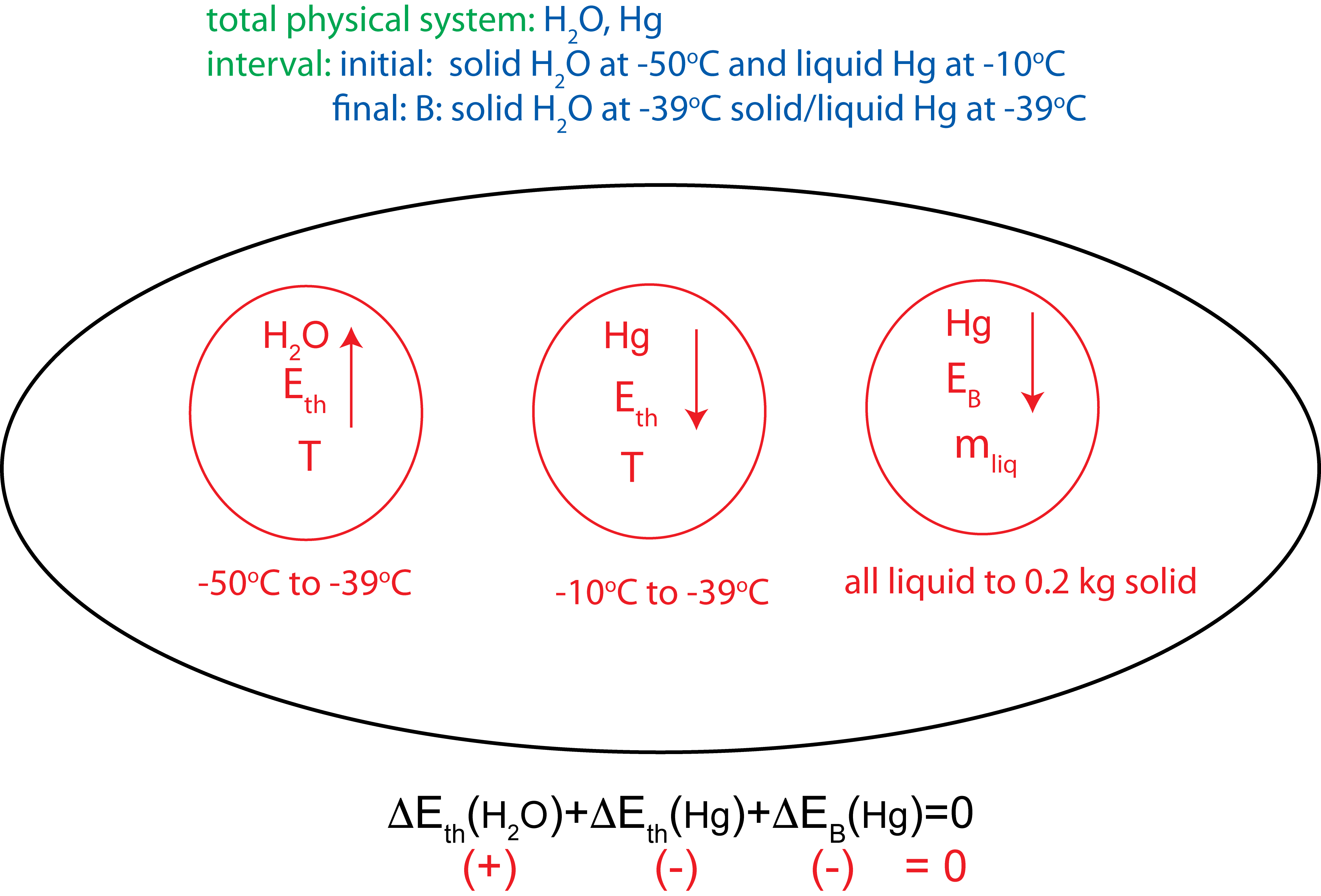
b) The equation of conservation of energy for this interaction is:

\(m_{ice}c_{ice}\Delta T_{ice}+m_{Hg}c_{Hg,liq}\Delta T_{Hg}-\Delta m_{Hg}\Delta H_{Hg,melt}=0\)

Solving for \(m_{Hg}\):

\(m_{Hg}=\frac{\Delta m_{Hg}\Delta H_{Hg,melt}-m_{ice}c_{ice}\Delta T_{ice}}{c_{Hg,liq}\Delta T_{Hg}}\)

Looking up the relevant values in Table 1.4.3, \(c_{ice}=2.05~kJ/Kkg\), \(c_{Hg,liq}=0.141~kJ/Kkg\), and \(\Delta H_{Hg,melt}=11.3~kJ/kg\). Plugging in numbers:

\(m_{Hg}=\frac{(0.2kg)(11.3~kJ/kg)-(0.5kg)(2.05~kJ/Kkg)(-39^{o}C+50^{o}C)}{(0.141~kJ/Kkg)(-39^{o}C+10^{o}C)}=2.22~kg\)

Once the system reaches equilibrium, there is 2.02kg of liquid Hg and 0.2kg of solid Hg, since the total mass is 2.22 kg.

 

Application to Chemical Reactions

Similar to substances going through phase transitions, chemical reactions involve breaking and forming of bonds. Thus, it seems logical that the concept of bond energy with the Energy-Interaction Model can be applied to various chemical reactions as well.

The bonds in reactants, chemical substances at the start of the reaction, break. While bonds in products, the resulting chemical substances in a reaction, form. Using the same arguments as we did for phase changes, forming bonds releases energy and breaking bonds requires energy. Thus, the change in bond energy of a chemical substance whose bond is broken is positive. When n number of moles of a chemical substance are broken, \(\Delta E_{bond}=n\Delta H\), where \(\Delta H\) is the enthalpy of the molecule. When a bond is formed the change bond energy is negative. For n moles of formed bonds, \(\Delta E_{bond}=-n\Delta H\). Chemical reactions can be exothermic when heat is transferred into the environment, thus, the total change in energy is negative. Other reactions are endothermic which require an input of energy, thus, the total change in energy is positive. One can determine whether a reaction is exothermic or endothermic by adding up all the total enthalpies of the reactants and subtracting the total enthalpies of the products:

\[Q=\Delta E_{tot}=\sum_i n_i \Delta H_{reactants}-\sum_i n_i\Delta H_{products}\]

For example, living cells use ATP as a source of energy for other reactions. The chemical reaction for ATP hydrolysis is shown here:

\[ATP+H_2 O\rightarrow ADP + P_i \]

A common misconception about ATP is that "breaking ATP releases energy". This statement is clearly inconsistent with what we have learned so far about bond energy, "breaking bonds requires an input of energy". So why do we say that ATP is the source of energy for life? Let us take a more careful look at this chemical reaction using the Energy-Interaction Model. When ATP and H₂O breaks down into its constituents, energy is required to break these bonds. However, when ADP and Pi are formed, energy is released.

The goal is to figure out whether this is an exothermic or an endothermic reaction and how much energy is either given off to the or taken from the environment. The Energy-Interaction diagram for the reaction (before performing the calculation) is shown below:

Figure 1.3.4: Energy-Interaction Diagram for ATP hydrolysis

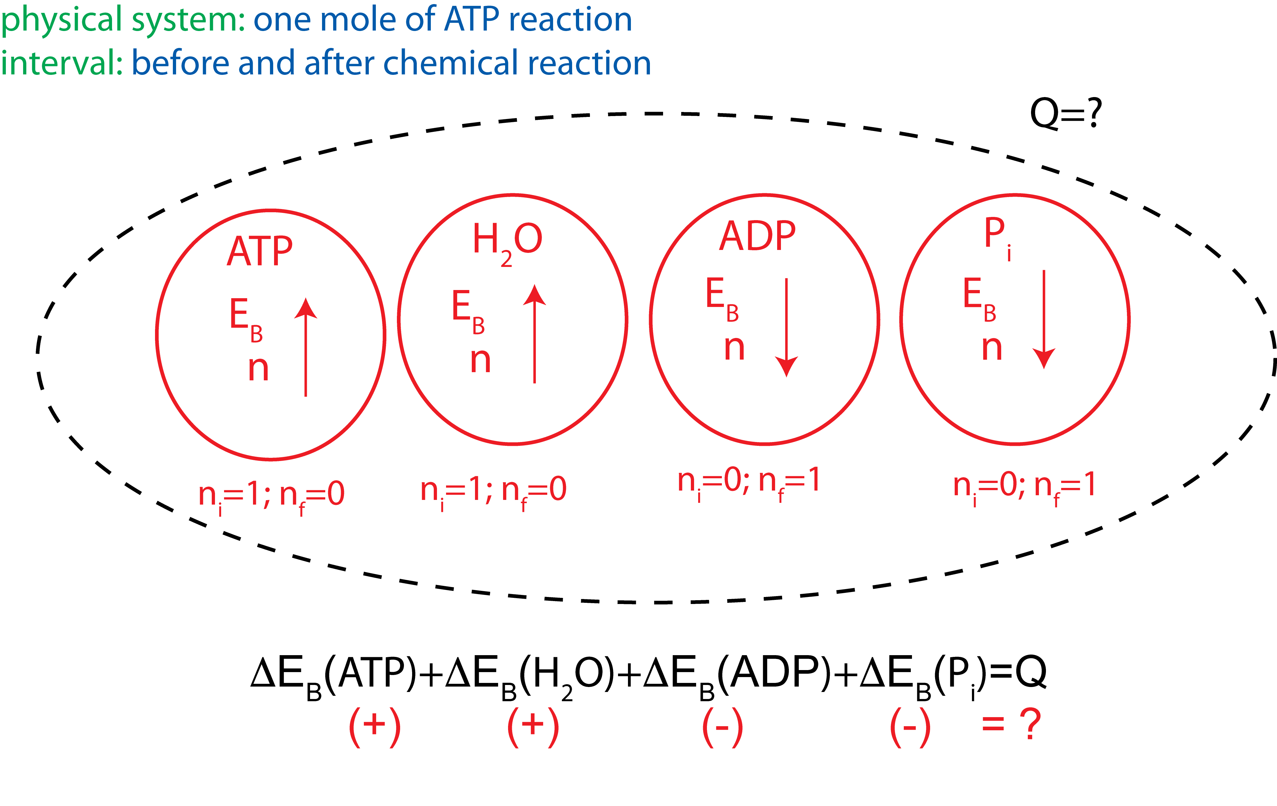
At standard conditions, \(|\Delta H_{ATP}|=2982~KJ/mol\), \(|\Delta H_{H_2O}|=287~KJ/mol\), \(|\Delta H_{ ADP}|=2000~KJ/mol\), and \(|\Delta H_{P_i}|=1299~KJ/mol\). Plugging into the above equation the enthalpy values for each molecule with the correct signs for the reactants and products we get: \(Q=2982+287-2000-1299=-30~kJ/mol\). This shows that the reaction is exothermic, so energy is released into the environment. Thus, although energy is required to break down ATP the net result of this reaction is production of energy. Now you can go back to the Energy-Interaction Diagram and modify it with heat, Q, leaving the system.