
2.6: Plotting Energies
- Page ID
- 19099
This page is a draft and is under active development.

Another Way to State Conservation of Energy
So far we have dealt only with changes in energy, since those are the important quantities for understanding the Energy-Interaction Model. In other words, what matters between two instances in time is how the energy of the system changed. However, sometimes it is useful to not only focus on two particular moments in time, but rather analyze energy over all instances in time. Recall, the energy-conservation equation for a closed system:
\[\Delta E_{tot}=0\]
This equation can be rewritten as:
\[E_{tot,final}=E_{tot,initial}\]
Since "initial" and "final" can refer to any instant in time as long as the system stays closed, the above equation implies that the total energy is constant over the entire interval:
\[E_{tot}=\text{constant}\]
Kinetic and Gravitational Potential Energy
Lets us return to the example depicted Figure 2.4.3 of a ball thrown upward. If we focus on the interval of the ball's path from the moment it was thrown upward to the moment it reached its maximum height, we can assume that the total energy is constant, as long as air friction is neglected:
\[E_{tot}=KE+PE_g=\text{constant}\]
which can be written as
\[E_{tot}=\frac{1}{2}mv^2+mgy=\text{constant}\label{totalE.ball}\]
This equation will hold for all values of y for which the ball/Earth system is closed. For example, if the ball falls back down and hits the ground, or if you catch the ball on its way down, the system would no longer be considered closed, since the ball/Earth would interact with another object (the floor or your hand). Also, the value of y cannot exceed the maximum height of the ball.
Equation \ref{totalE.ball} is informative, but it is often instructive to represent physical behavior graphically. We would like to make a plot of KE and PEg as a function of height. In order to make this plot we need to define a physical location that represents the origin of y (where is y=0?). Since we want to plot the interval from the moment the ball is thrown to its maximum height, the logical location of the origin is the location of the ball right after it is thrown, as shown in the figure below.
Figure 2.6.1: Setting the origin of y for the ball thrown upward.
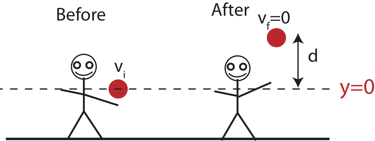
The gravitational potential energy in this interval will vary linearly with y, from \(PE_g=0\) at y=0 to \(PE_g=mgd\) at y=d. Next, we can find the total energy. We know that at the maximum height the speed of the ball will go to zero. Thus, \(KE=0\) when y=d, and:
\[E_{tot}=PE_g+KE=mgd\]
Once we know the total energy in one location, we know it everywhere when the system is closed, since the result above tells us that \(E_{tot}=\text{constant}\). To find how KE changes with height we can then use, \(KE=E_{tot}-PE_g=mgd-mgy\). This equation tells us that KE will vary from \(KE=mdg\) at y=0 to \(KE=0\) at y=d. The plot describing these results is shown below.
Figure 2.6.1: Energy plots of for a ball thrown upward

Note, that our choice of "zero" was just a convenient choice, which resulted in the particular plot of PEg and Etot shown in the figure. (Kinetic energy does not depend on the choice of the origin, since its indicator is speed.) There was nothing physical about this choice, we could have as well chosen the maximum height, the ground, or the center of the Earth as "zero" height. The different choices would result in different values of potential energy, and thus different total energy values. It is even possible to have negative values of PEg and Etot as we saw in the vertical spring example in the previous section. Potential energy depends on location of the system, thus, it will depend on the choice of origin. However, regardless on where you choose to define zero, the changes in energies for a given interval will always be the same. The physical meaning is contained in the relative position between two points in space.
Alert
Although initially it might seem very counterintuitive to your understanding of energy, there is nothing unphysical about a system having negative energy. It is very important to think about energy as a property of the system that changes when there is an interaction that happens. The potential energy of the system depends on position. In order to assign a value for position an origin needs to be defined. Since the definition of the origin is arbitrary, the values of potential energy will be arbitrary as well. What does stay the same is how that potential energy changes. When you lift an object 1m up from the ground, the change in height will be 1m whether you lifted it from y=0 to y=1m or from y=-1m to y=0m.
Example \(\PageIndex{1}\)
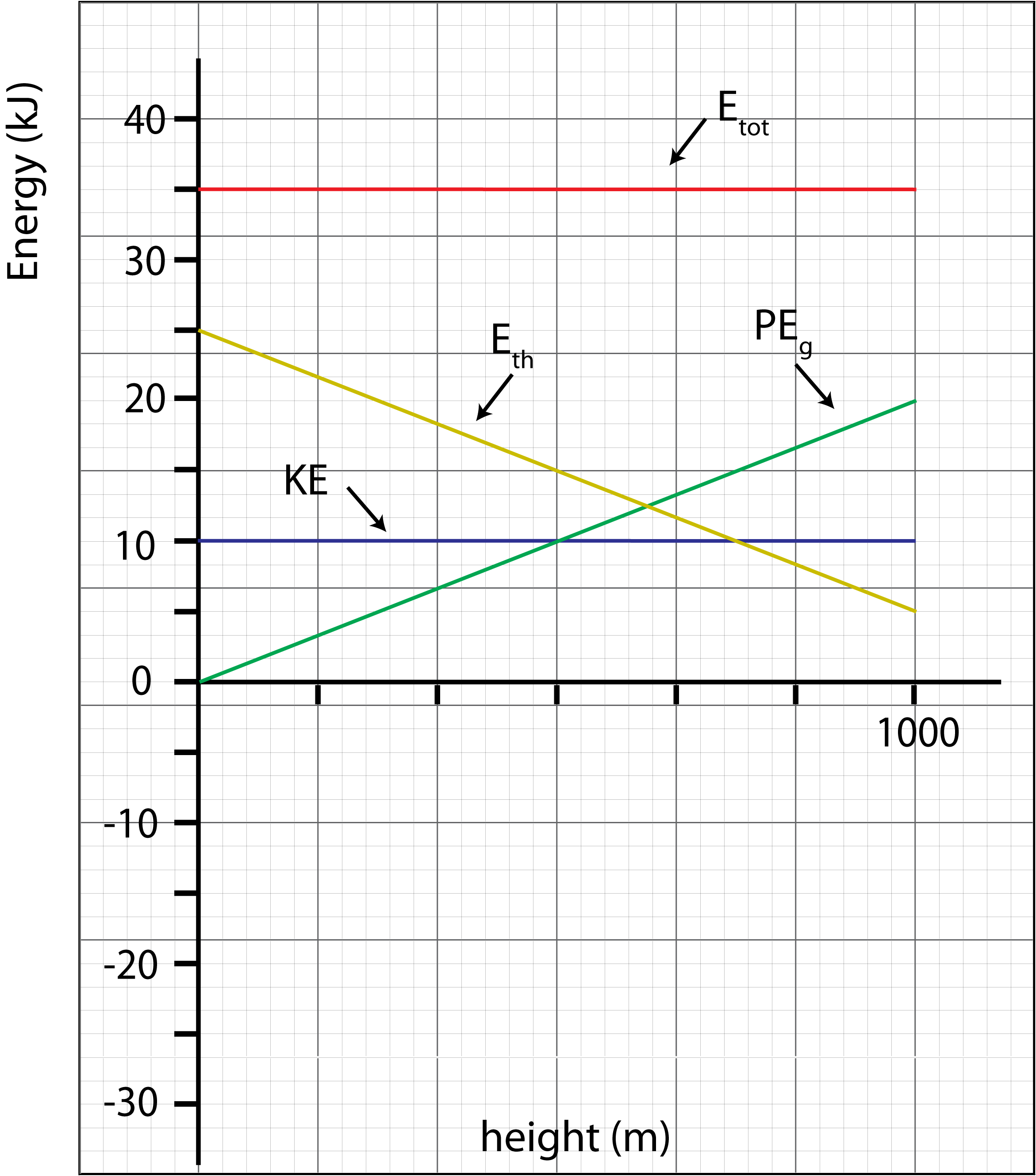
A 2kg meteorite enters Earth’s atmosphere. At an altitude of 1000 meters it is traveling at terminal velocity (constant speed) of 100 m/s. The total energy of the meteorite/earth/air system is 35KJ during an interval from when the meteorite is 1000 meters high to right before it hits the ground. Plot all the energies involved: total energy, kinetic energy, gravitational potential energy, and thermal energy as a function of height from y=0 meters (defined to be the ground) to y=1000m in the air.
- Solution
-
Since the meteorite is falling (PEg is decreasing) but the speed is staying constant, there must be friction present to account for loss of mechanical energy. This is friction of the meteorite and air, air friction. The total energy of this system is:
\[E_{tot}=PE_g+KE+E_{th}\nonumber\]
At 1000m: \(E_{tot}=35kJ\), \(KE=\frac{1}{2}mv^2=\frac{1}{2}(2kg)(100)^2=10kJ\), \(PE_g=mgy=(2kg)(9.8m/s^2)(1000m)=19.6kJ\), and \(E_{th}=E_{tot}-KE-PE_g=4.6kJ\)
At 0m: \(E_{tot}=35kJ\), \(KE=10kJ\), \(PE_g=0kJ\), and \(E_{th}=25kJ\)
The plot below shows all energies in this interval.
Spring-Mass Systems: a Universal Motion
Most physical systems that vibrate back and forth do so like a hanging spring-mass, particularly when the amplitude of vibration is not too large. Because this motion is so common and so important in understanding a lot of physics, it is worth looking at it a little closer.
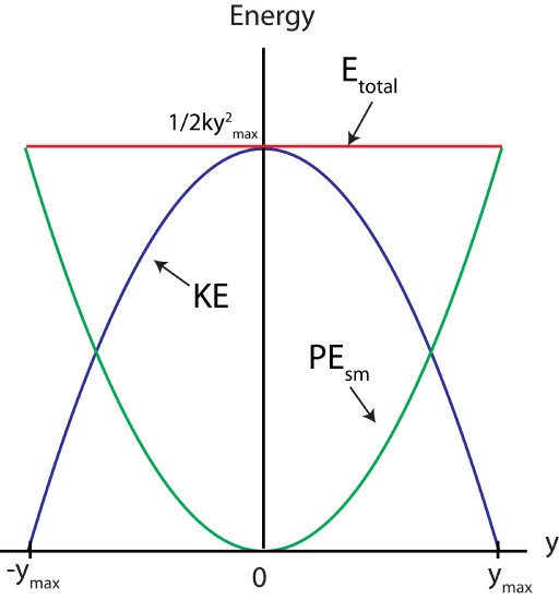
As we saw in the previous section, the maximum value of the PEsm of the spring-mass system occurs when the mass is at its extreme positions (maximum displacement from equilibrium), and its speed is zero. Conversely, the KE of the spring-mass system is a maximum when the mass is at its equilibrium position (y=0). When the system is closed in the absence of friction, \(\Delta E_{tot} = \Delta KE + \Delta PE_{sm}=0\), or equivalently Etot is a constant. Looking at Etot at any particular time in its cycle of vibration, the energy is still going to be equal to the same total value. Written symbolically (we chose "y" to represent a vertical spring-mass, but the choice of variable is arbitrary):
\[E_{tot} = PE_{sm} + KE =\frac{1}{2}ky^2+ \frac{1}{2}mv^2=\text{constant} = PE_{max} = KE_{max}\]
Since the dependence of PEsm on displacement y is quadratic, the function will be parabolic. The total energy is the energy when the spring is at its maximum displacement, \(E_{tot}=\frac{1}{2}ky_{max}^2\). The kinetic energy as a function of y is the difference between the maximum energy, Etot and PEsm, \(KE=E_{tot}-PE_{sm}\). The graph below shows the kinetic energy KE and potential energy PEsm of a spring-mass system as a function of the position from equilibrium, y.
Figure 2.6.2: Energy plots of for a spring-mass system
Although we cannot show it without investigating the time behavior of the motion of the mass, it turns out that the time-average (that is, the average over time) of PEsm and KE are the same, and are consequently both equal to one-half the total energy:
\[\text{avg } KE_{spring-mass} = \text{ avg } PE_{sm} = \dfrac{1}{2}E_{total} \]
The fact that the time-average potential and kinetic energies are the same has a profound implication for the model of matter that we are about to develop in Chapter 3. This result is true only for a potential energy that depends on the square of the variable. It is precisely the fact that the potential energy is quadratic with respect to position that makes a spring-mass system so special, so universal, and so important.
The lowest point on the PEsm curve is frequently called the potential energy minimum. Why is the value of the position variable for which the potential energy is a minimum significant? Consider what happens as energy is removed from a system which is oscillating about the equilibrium value of its position (e.g., a real spring-mass system, because of friction, gradually transfers mechanical energy to thermal energy). The amplitude (maximum extent) of the oscillations decreases until eventually, when all mechanical energy has been transferred to thermal systems, the system comes to rest at the equilibrium position, the position of the potential minimum.
Now consider any physical system that oscillates and which will settle down to a stable position as energy is transferred to thermal systems. That stable equilibrium position represents the physical state where potential energy is smallest. (All of the PE and KE have been transferred to thermal systems.) The potential energy must increase as y increases (either positively or negatively) away from zero, the equilibrium position. Now nature seems to prefer smooth changes of things like potential energies. The simplest smooth mathematical function that increases for both positive and negative y is y2. When we look at real physical systems, it turns out that sufficiently close to the minimum, the potential energy always “looks parabolic”! This is a result with far reaching consequences. It implies that any oscillating system behaves just like our simple spring-mass system, at least for small amplitudes of oscillation! What’s important is not that the spring-mass system is so special itself; it is, rather, that the behavior of the spring-mass system represents a truly universal behavior of any oscillating system and oscillating systems are found everywhere in nature. We will use this property in Chapter 3 when we model the real atoms of liquids and solids as “oscillating masses and springs”.