
5.7: The Linear Transport Model
- Page ID
- 17166

Steady-State Transport Phenomena
We have extensively described two different systems whose behavior can be described with a steady-state transport model, flowing fluid and moving electric charge systems. In both systems, we saw that to have a current there has to be a energy-density difference between two locations in space, such as a voltage or pressure difference. In this section we will generalize this phenomena to other systems that behave in this matter. In the next section we will look at a non steady-state transport model, where current is no longer constant as a function of time.
We generalize the difference in pressure or voltage, or a driving potential that causes current to a gradient, which means change in the quantity with change in position. For fluid flow there must be a gradient in the total head. In order to have electric charge flow, there must be a gradient in the electric potential. In each case, the flow is proportional to the inverse of the resistance.
The transport equations for fluids and current electricity (without pumps or batteries) and using the subscripts “F” to denote fluids and “E” to denote electric charge become:
\[\Delta\text{(total head)}=– I_F R_F\]
\[\Delta V=– I_E R_E\]
And solving for \(I\) results in:
\[I_F=-\dfrac{\Delta\text{(total head)}}{R_F}\]
\[I_E=-\dfrac{\Delta V}{R_E}\]
For any system that abided by this behavior, we can define a general potential, \(\phi\). Then, the current, \(I\) due to the gradient, \(\Delta\phi\) is defined as:
\[I=-\dfrac{\Delta\phi}{R}\label{I-gen}\]
There are many phenomena that involve the motion or transport of some quantity that behave similarly to the way fluids and electric charge flow in those sections of a circuit without sources of energy density (pumps or batteries). In steady-state, after all transients have settled out, we can model these phenomena the same way we model fluids and electric charge flow. These are such common and general phenomena that it is useful to collect them together under their own specially named model, the linear transport model.
This model has the following main components:
- a current describing flow as a function of time.
- a gradient causing current.
- resistance impeding the flow.
- the gradient is proportional to current and inversely propositional to resistance.
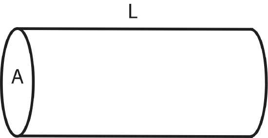
Resistance to flow is typically depends on the material and the geometry of the medium. It can be written in terms of conductivity, \(k\), which characterizes the specific material such as a steel or plastic pipe, the cross sectional area of the pipe, the wire, or whatever is constraining the flow, \(A\), and the length of the circuit under consideration, \(L\).
\[R = \dfrac{1}{k}\left(\dfrac{L}{A}\right)\label{R}\]
This relation says that the resistance increases with the length of the pipe or wire, is inversely proportional to the cross-sectional area, and is inversely proportional to the conductivity of the pipe or wire.
Figure 5.7.1: Flow through a pipe of length \(L\) and cross section \(A\).
Plugging this into the expression for current in Equation \ref{I-gen} we get:
\[I=-k\dfrac{A}{L}\Delta\phi\]
We can generalize these relations further by defining the flux \(j\), whihc is the amount of what is flowing that passes a unit area per unit time.
\[j = \dfrac{I}{A}\]
Then the expression for \(j\) becomes:
\[j = – \dfrac{k}{L} \Delta \phi \label{Eq5}\]
Our final generalization is to imagine the length, \(L\), shrinking down to infinitesimal size, so that \(\Delta \phi\)/L becomes simply the derivative of the potential d\(\phi/\)dx in the direction of the flow, called the gradient of the potential. Hence
\[\lim_{L\to 0}\dfrac{\Delta \phi}{L} = \dfrac{d\phi}{dx} \label{Eq6}\]
Thus Equation \(\ref{Eq5}\) turns into a generalized linear transport equation:
\[j = – k \dfrac{d \phi }{dx} \label{genlinEQ}\]
In words this relation says that the flux of whatever it is that flows is proportional to a constant that depends on the characteristics of the physical system, which is the conductivity for fluids and electric current and to the gradient of the potential. The faster the potential changes in the direction of the flow, the higher the flow. The gradient of the potential is the driving force that causes the fluid or electric charge to flow in the presence of the resistance. Thinking back to our energy-density model, the gradient of the potential is simply the change (loss) in fluid or electric energy density as you move along with the flow. The minus sign is consistent with the convention that the flux is positive in the direction of flow. Because the gradient of the potential is negative in the direction of flow, the extra minus sign in the relation, makes the flux positive.
The units of the flux and current, conductivity, and potential depend on whatever it is that is flowing. We now look at several specific cases. To get an expression in terms of resistance, we use the relation in Equation \ref{R}.
Fluid Flow
We consider a current flowing through a round pipe of radius \(r\), cross sectional area \(A\) and length \(L\). If the flow is in the low-velocity regime (streamline or laminar flow) the expression for resistance is simply the product of two factors. One factor incorporates pipe geometry and the other incorporates fluid properties. We can intuitively see how geometry, the length and area of the pipe (or other similar structure) influences resistance. If fluid flows through the pipes that differ only in length, the longer one will have more loss to the thermal energy-density. If two pipes differ in cross-sectional area, the pipe with the smaller area will have a greater proportion of fluid interacting with the pipe walls, and thus will lose more energy to the thermal energy-density.
Incorporating pipe geometry properties with a fluid property, viscosity, \(\eta\), we have the following relations:
\[R = (\text{fluid properties}) \times (\text{geometry properties}) \]
\[R= 8 \eta \times \dfrac{L}{Ar^2} \]
Note the very strong dependence of flow resistance on the radius of the pipe or tube: inversely proportional to the fourth power of the radius. This has interesting consequences in many common situations, including partially clogged water pipes and arteries. Viscosity has units of \(Js/m^3\). A table of viscosities for several fluids is given below.
| Fluid at specific temperature | viscosity, \(\eta\) (Js/m3) |
|---|---|
| air (20° C) | \(1.8 \times 10^{-5}\) |
| water (20° C) | \(1.8 \times 10^{-3}\) |
| water (20° C) | \(1.0 \times 10^{-3}\) |
| water (90° C) | \(0.32 \times 10^{-3}\) |
| blood (37° C) | \(4 \times 10^{-3}\) |
| light motor oil (20° C) | \(0.03\) |
| glycerin (20° C) | \(1.5\) |
When the velocity of the fluid is high, the flow is turbulent, a chaotic and irregular flow. The value of the resistance when flow is turbulent is always greater than for smooth streamline (laminar) flow. Because it is complicated to model and not independent of velocity, we won’t discuss turbulent flow quantitatively in this course. It is useful to know, however, in case you encounter fluid flow in your future studies, that it is possible to calculate a particular parameter, which is a function of current, fluid properties as well as dimensions and shape of the pipe, that allows one to roughly predict whether laminar or turbulent flow will occur. This dimensionless parameter is called the Reynolds number. The flow is laminar for values of the Reynolds number less than about 2000 and turbulent for values greater than about 3000. The flow is unstable for intermediate values. For now, the important point to remember is simply that as flow velocity increases, the flow will eventually become turbulent and the resistance will increase significantly. This phenomenon of increasing resistance occurs in many common fluid systems including air moving in the ductwork in forced-air heating and air conditioning systems, water flowing in typical household water distribution systems, and blood flowing in arteries.
Electric Charge Flow
As with the resistance to fluid flow through pipes, the resistance to the movement of electric charge can be separated into a factor dependent solely on the geometry of the material through which charge moves and another factor independent of geometry, but dependent on the details of the charge carriers and how they interact with the material through which they move.
Focusing first on the geometry factors, the resistance will increase proportionally with the length, \(L\), and the inverse of the cross sectional area, \(A\). In fluid flow, the geometry independent factor is a property of the fluid itself, viscosity; in charge flow it is a property of the material through which the charge flows. This geometry independent factor is called resistivity, \(\rho\), which is the reciprocal of the conductivity, \(k=1/\rho\). From Equation \ref{R} we can determine that the units of conductivity are \(1/\Omega m\), thus, the units of resistivity are \(\Omega m\). Combining the two factors, the resistance is:
\[R =\dfrac{1}{k}\dfrac{L}{A}=\rho\dfrac{L}{A}\]
Shown below is a table of resistivities for various materials. Substances that have high conductivities (low resistivities) are good electrical conductors. Metals are usually good electrical conductors. Substances that have low conductivities (high resistivities) are said to be good insulators. Glass and most plastics are good insulators. Note the extremely large range of resistivities for common materials. In most materials there is a small dependence of resistivity on temperature. In semiconductors the dependence of resistivity on temperature is typically larger than for insulators or metals. A strong current dependence arises if the thermal heating, due to the resistance, causes the temperature of the material to increase substantially. This is the case with ordinary tungsten light bulbs, the kind that get hot. The resistance of the filament of these light bulbs increases many times as they go from room temperature to their typical operating temperature, which is several thousand degrees.
| Material | Electric Resistivity, \(\rho\) (\(\Omega\)m) |
|---|---|
| glass | \(10^{10}-10^{14}\) |
| diamond | \(2.7\) |
| silicon | \(2.5 \times 10^{3}\) |
| mercury | \(96 \times 10^{-8}\) |
| iron | \(10 \times 10^{-8}\) |
| turngsten | \(5.5 \times 10^{-8}\) |
| aluminum | \(2.8 \times 10^{-8}\) |
| copper | \(1.7 \times 10^{-8}\) |
| silver | \(1.6 \times 10^{-8}\) |
| fat | \(25\) |
| blood | \(1.5\) |
| saturated NaCl solution | \(0.044\) |
Heat Flow
In heat conduction, the quantity that flows is heat which transfers thermal energy. We are imagining a non-equilibrium situation in which the temperature is hotter at one end of a rod, for example, than at the other end. The driving potential is the gradient of the temperature in the material. The "current” is the heat per time, which is power. Power in heat flow is analogous to the current in fluid or charge flow. Here, power is the amount of thermal energy that is transferred per second past a plane which is oriented perpendicular to the gradient of the temperature. The thermal flux is the power per unit area. Heat flows due to a temperature gradient within a solid, liquid, or gas.
For heat flow in the generalized transform Equation \ref{genlinEQ}, \(k\) is the thermal conductivity in units of Watts per meter Kelvin, \(W/mK\), and \(d\phi /dx\) becomes the temperature gradient in units of Kelvin per meter, \(K/m\). Flux is power per unit area resulting in:
\[\dfrac{P}{A} = – k \dfrac{dT}{dx}\]
For an object (window pane perhaps) with cross sectional area \(A\), thickness \(L\), and temperature difference across the surfaces,\( \Delta T\), the total heat transported across the object would be:
\[P = – k A \dfrac{ \Delta T}{L}\]
Metals that are good electrical conductors are usually also good thermal conductors. This is because the movement of “free” electrons in the metal is primarily responsible for both electrical and thermal conduction. However, the vibrations of atoms can also transport thermal energy with little resistance, provided the material is very pure. Diamond is an electrical insulator; its electrons are strongly bound to the carbon atoms and are not free to transport electric charge. However, diamond has a thermal conductivity considerably larger (thermal resistivity smaller) than any metal at room temperature! List of materials and their thermal conductivities is given in the table below
| Material | Thermal Conductivity, k (W/mK) |
|---|---|
| down | \(0.02\) |
| air | \(0.026\) |
| Styrofoam | \(0.03\) |
| fiberglass | \(0.04\) |
| water | \(0.0597\) |
| human tissue (no blood) | \(0.21\) |
| fat | \(0.17\) |
| glass | \(0.7-1.0\) |
| wood | \(0.1\) |
| lead | \(35\) |
| iron | \(74\) |
| aluminum | \(235\) |
| copper | \(400\) |
| silver | \(427\) |
| diamond | \(990\) |
We see from the table that air is an extremely poor conductor of heat (as long as there is no convection; i.e., macroscopic movement of the air), which makes it an excellent insulator. When you bundle up on those ski trips in the mountains, it is most effective to trap air between you and your outerwear with a wool sweater and/or long johns, and wear a down or Holofil™ jacket with many microscopic pockets of trapped air. The walls and roofs of our houses are layered with fiberglass mats or similar material that are designed to trap air in order to be effective insulators. Double-pane windows also trap "dead air" between the outside environment and the inner window.
Diffusion
There are many phenomena in various branches of science that are generally referred to as diffusion. In its basic form, diffusion is simply the net motion (net transport) of a particular species of particles that is due to the presence of random thermal motion that naturally exists at all temperatures above \(0 K\) and due to to the presence of a concentration gradient of that species of particle. Diffusion of particles occurs in solids, liquids, and gases. Another common example occurs when permeable or semipermeable membranes are present. If a concentration difference of some particle species exists across a membrane that is permeable to those particles, then there will be a flow of those particles across the membrane from the region of high concentration to the region of low concentration. If the concentration gradient is removed, transport ceases. The greater the concentration gradient, the greater the number of particles transported per unit time.
Steady-state diffusion is described by the linear transport model. We re-write the generalized linear transport equation as:
\[j = – D \dfrac{dc}{dx}\]
This is historically known as Fick's Law. The letter, \(D\) is the diffusion constant. In SI units of square meters per second, \dfrac{m^2}{s} \), \(c\) is the particle concentration in SI units of number per cubic meter, \(1/m^{-3} \), and \(\dfrac{dc}{dx}\) is the particle concentration gradient in SI units of \(1/m^{-4}\). The particle flux, \(j\), has units of number per square meter second, \(1/m^2s\). The units of \(j\) and \(D\) are often expressed in terms of moles rather than number of particles.
Values of diffusion constants range over many orders of magnitude. The diffusion of nuclear magnetization (due to the very weak magnetic moments of nuclei) in pure insulating crystals can be as small as \(1.0 \times 10^{-17} m^2s^{-1}\) while the diffusion of hydrogen in air at STP is nearly \(1.0 \times 10^{-4} m^2s^{-1}.\) The table below lists some representative values of solute-fluid combinations at 20°C and 1 atm pressure.
Table 5.7.4: Diffusion constant for various solutes in various media.
| Solute | Medium | Thermal Conductivity, D (m2/s) |
|---|---|---|
| oxygen | water | \(1.0\times 10^{-9}\) |
| oxygen | air | \(1.8\times 10^{-5}\) |
| oxygen | tissue | \(2.0\times 10^{-11}\) |
| hydrogen | air | \(6.4\times 10^{-5}\) |
| glucose | water | \(6.7\times 10^{-10}\) |
| sucrose | water | \(5.0\times 10^{-10}\) |
| hemoglobin | water | \(6.9\times 10^{-11}\) |
| DNA | water | \(1.3\times 10^{-8}\) |
| pollen grain | water | \(1.0\times 10^{-12}\) |
In steady state conditions, the linear transport model using the constructs of concentration and concentration gradient works well. However, in transient conditions, a better approach is to use the mobility, rather than concentration, and the free energy gradient, rather than the concentration gradient in the linear transport equation. This latter approach avoids having to let the diffusion constant be a function of the concentration.
Other Examples of Linear Transport
As previously indicated, there are many transport phenomena that can be understood with the linear transport model. Many of these phenomena have been given special names (laws). It is easy to not realize that they are all understandable from the general perspective of the linear transport model. For example, in studying subsurface water flow Henry Darcy established in the 1850’s with a series of sand column experiments that, for a given type of sand, the volume flow rate, i.e., the current I, was proportional to the head difference and cross-sectional area of the column and inversely proportional to the column length. From what you know about linear transport, you should be able to predict the law that bears his name, Darcy’s law, simply by assuming that there is a soil-dependent conductivity (known today as the hydraulic conductivity of the soil) and writing down the general linear transport equation:
\[\dfrac{I}{A} = k_{soil} \dfrac{d(head)}{dx}. \]
Summary
A summary of the algebraic relationships and relationships in Linear Transport Model as it applies to fluid flow, current electricity, heat conduction and diffusion is given here.
Flux:
\(j = \dfrac{I}{A} \)
Generalized linear transport equation:
\(j = – k\dfrac{d \phi }{dx}\)
Relationship of resistance, R, conductivity, k, and resistivity, \(\rho\) :
\(R = \rho \dfrac{L}{A}~~k = \dfrac{1}{\rho}\)
Table 5.7.5: Summary and Comparison of Several Steady-State Transport Systems
| Parameter | Laminar Fluid Flow | Electric Flow | Heat Conduction | Diffusion |
|---|---|---|---|---|
|
Transported quantity |
Fluid Volume: \(V\) [\(m^3\)] |
Electric charge, \(q\) [\(C\)] |
Heat, \(Q\) [\(J\)] |
Particles, \(n\) [number or mol] |
|
Current |
Volume per unit time: flow rate \(I\) [\(m^3/s\)] |
Charge per unit time: electric current \(I\) [\(C/s\)], or [\(A\)] |
Heat per unit time: power \(P\) [\(W\)] |
Particle number per unit time: particle current \(I\) [\(1/s\)] |
| Flux: \(j=\dfrac{I}{A}\) | [\(m/s\)] | [\(A/m^2\)] | [\(W/m^2\)] | [\(1/m^2s\)] |
| Potential, \(\phi\) |
Total head: energy per unit volume [\(J/m^3\)] or [\(N/m^2\)] or [\(Pa\)] |
Voltage, \(V\): energy per unit charge [\(J/C\)] or [volts, \(V\)] |
Temperature, \(T\): [Kelvin, \(K\)] |
Particle concentration, \(c\): [\(1/m^3\)] |
|
Potential gradient: \(\dfrac{d\phi}{dx}\) |
\(\dfrac{d (\text{head})}{dx}\) [\(J/m^4\)] |
\(\dfrac{dV}{dx}\) [\(V/m\)] |
\(\dfrac{dT}{dx}\) [\(K/m\)] |
\(\dfrac{dc}{dx}\) [\(1/m^4\)] |
|
Conductivity: (inverse of resistivity) |
Fluid conductivity, \(k\) [\(m^5/Js\)] |
Electric conductivity, \(k\) [\(1/\Omega m\)] |
Thermal conductivity, k [\(W/Km\)] |
Diffusion constant, \(D\) [\(m^2/s\)] |
| Transport Equation | \(j=-k\dfrac{d(\text{head})}{dx}\) | \(j=-k\dfrac{dV}{dx}\) | \(j=-k\dfrac{dT}{dx}\) | \(j=-D\dfrac{dc}{dx}\) |
Contributors
Authors of Phys7B (UC Davis Physics Department)