3.4: Single-Slit Diffraction

Slits Are Not Actually Point Sources

In our discussion of the double slit and diffraction grating, we made the assumption that the gaps that we call slits are so narrow that they can essentially be treated as point sources, making the analysis using Huygens's principle simple to do. But in reality we know that these gaps do not have infinitesimal width, and we need to consider what happens to the light when the approximation of "very thin gaps" breaks down. To do so, we will not consider a grating, or even a double-slit; we'll look at the effect that a single slit of a measurable gap size has on the light that passes through it. Notice that whatever this effect might be, when we extend the result to two or more slits, the effect will occur for every slit, superimposing itself on the multiple-slit interference pattern. But we are getting ahead of ourselves...

We already know that a plane wave passing through a single slit will diffract around the corners, so it will not simply leave a single bar of light on the screen the thickness of the gap – it will spread out. But what else can we say about it? Well, we know that without the aperture, all the Huygens wavelets would continue interfering perfectly to continue the plane wave, but when the portions of the plane wave outside the aperture are excluded, the effects of interference between wavelets is bound to change. We will analyze the effect by essentially following the procedure for many (infinite number) of thin slits that are infinitesimally close together.

Single Slit Interference Pattern

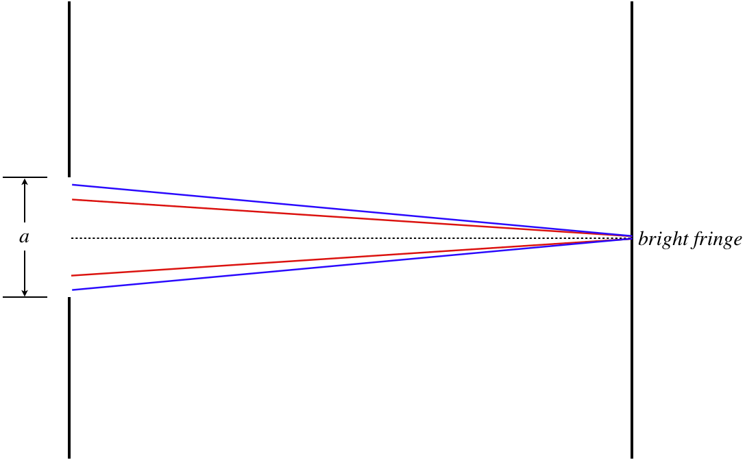
Let's call the gap width of the aperture \(a\), and assume that this is much smaller than the distance to the screen, as in the figure below. We then consider what happens to the wavelets originating from every point within this region. When we look at how the screen opposite a single slit is illuminated, on the screen at the center line we observe a brightness maximum. You can think of such a situation as an infinite number of double-slits that are split by the center line with different slit separations. For every wavelet above the center line, there is a "twin" wavelet on the opposite side of the center line that travels the same distance to the screen (depicted by lines of the same color in the figure below), resulting in constructive interference. Of course, the fact that pairs constructively interfere with each other does not guarantee that the result of two constructively-interfering wavelets will not cancel with two other constructively-interfering wavelets (i.e. one pair creating a doubly-high peak, and the other a doubly-deep trough). In fact this can happen, but if it does, it's only for select wavelets – it can't persist for the entire aperture and leave darkness at the center line. Without going into the math, wavelets find it exceedingly difficult to find canceling partners at the center line, and on balance the interference is highly constructive – the center line is the brightest point in the entire interference pattern.

Figure 3.4.1 - Wavelet Pairs Constructively Interfere at the Center Line

Okay, so what about dark fringes – will we see these on the screen? Yes! To see why, we will once again find pairs of wavelets on both sides of the center line, which in this case travel different distances to the screen, differing by one-half wavelength for the first dark fringe. For this case, we pair-off the wavelet originating at the top of the slit with the wavelet originating just below the center line, and continue pairing them as we go down, until the wavelet at the bottom edge pairs with the wavelet originating just above the center line. This is depicted in the figure below with pairs of lines of the same color. The difference in distances for these pairs will all be the same (\(d\sin\theta\), where in this case \(d\) is actually \(\frac{a}{2}\)), and when this difference is one-half wavelength, they all cancel each other pairwise, leaving a dark fringe.

Figure 3.4.2 - Wavelet Pairs Destructively Interfering at the First Dark Fringe

Note that the same geometry holds below the center line as well. Setting the extra distance traveled by the twin wavelets equal to a have wavelength, we get the angle of the first dark fringe:

\[\text{first dark fringe:}\;\;\;\;\;\dfrac{a}{2}\sin\theta = \dfrac{\lambda}{2} \;\;\;\Rightarrow\;\;\; \sin\theta = \pm \dfrac{\lambda}{a} \]

As we move upward on the screen, wavelets will again find their destructive twins and create dark additional dark fringes. It is a bit tricky for us to find the second dark fringe, however. The natural approach is to assume that the next dark fringe occurs when the pairs shown above travel distances that differ by three half-wavelengths, giving the result \(\sin\theta = \pm 3\frac{\lambda}{a}\). But in fact this result incorrectly skips the second dark fringe, and goes to the third! To see why, we note that we can pair-off wavelets in a way other than across the center line. Specifically, we can think of this single slit as two adjacent single slits, one that has the center line as its lower edge, and one that has the center line as its upper edge. In this case, the wavelets pair-off within the top half, and then again within the bottom half separately. In this case, the only change in the math involves replacing \(\frac{a}{2}\) with \(\frac{a}{4}\), which means the second dark fringe satisfies:

\[\text{second dark fringe:}\;\;\;\;\;\dfrac{a}{4}\sin\theta = \dfrac{\lambda}{2} \;\;\;\Rightarrow\;\;\; \sin\theta = \pm 2\dfrac{\lambda}{a} \]

We can similarly break the slit into three separate slits, which changes the separation of the starting wavelets to \(\frac{a}{6}\), and increments the constant in the formula to 3. For the \(m^{th}\) dark fringe, we therefore have:

\[m^{th}\text{ dark fringe:}\;\;\;\;\;\sin\theta = \pm m\dfrac{\lambda}{a} \]

The bright fringes only approximately follow the same spacing pattern, not exactly located halfway between the dark fringes, but using the pairwise approach doesn't tell us much about the intensity of those bright regions, for the same reason it didn't for the central bright fringe – constructive pairs will not be in phase with other constructive pairs. Significantly more math is required to deal with the intensity of the bright fringes.

Intensity

To compute the intensity of the interference pattern for a single slit, we treat every point in the slit as a source of an individual Huygens wavelet, and sum the contributions of all the waves coming out at an arbitrary angle. One way to think of this is to go back to the diffraction grating case, expressed in Equation 3.3.2. With the slit being completely open, however, the space between the slits (\(d\)) goes to zero, and the number of slits (\(n\)) goes to infinity. There is of course more to the calculation than this, and either the calculus or the "phasor method" described by many standard physics textbooks will reach the famous result below, and the reader is encouraged to have a look at these derivations. But these derivations do not contribute to the understanding of this phenomenon, nor are they procedures essential to a wide range of future physics calculations, so we will omit them here, and jump to the end result.

If we define the amplitude of the total wave on the center line to be \(A_o\) due to the superposition of all the wavelets, then the amplitude of the wave at an angle \(\theta\) off the center line is given by:

\[A\left(\theta\right) = \dfrac{\lambda A_o}{\pi a\sin\theta}\sin\left(\frac{\pi a\sin\theta}{\lambda}\right)\]

Yes, you are reading that right, there is a sine function of \(\theta\) within another sine function. This is often written more succinctly by defining a new variable that is an implicit function of \(\theta\):

\[A\left(\alpha\right) = A_o\dfrac{\sin\alpha}{\alpha},\;\;\;\;\; \alpha\left(\theta\right)\equiv \dfrac{\pi a}{\lambda} \sin\theta \]

This function comes up frequently enough in math and physics that it has even been given its own name – it is sometimes referred to as a sinc function.

Alert

It is important to understand that this expression compares the amplitude at various angles to the amplitude on the center line, equal (or approximately equal) distances from the slit. It does not provide a comparison of the amplitude of the light wave after passing through the slit to the amplitude of the plane wave before it enters the slit.

We know that the intensity of the wave at the center line is proportional to the square of the amplitude there, and that the intensity of the wave at an angle with the center line is proportional to the square of the amplitude there, and that the constants of proportionality are the same in both cases, so we immediately have a comparison of intensities:

\[I\left(\alpha\right) = I_o \left[\dfrac{\sin \alpha}{\alpha}\right]^2 \]

If the angle \(\theta\) happens to be small, then \(\alpha\) can be written as a function of distance \(y\) from the center line on the screen, as we did in Equation 3.2.5 for the double slit, giving:

\[\alpha\left(y\right)\equiv \dfrac{\pi a y}{\lambda L}\;, \]

where, as before, \(L\) is the distance from the slit to the screen.

Perhaps you are concerned about the behavior of this function at the center line? After all, the value of the function \(\alpha\) there does vanish, and this function appears in the denominator. But the numerator also vanishes at the center line, and L'Hôpital's Rule saves the day, giving the sinc function a value of 1 for \(\alpha = 0\), resulting in the intensity equaling \(I_o\), as it should.

A graph of the intensity of the full interference pattern looks like this:

Figure 3.4.3 - Single Slit Diffraction Intensity

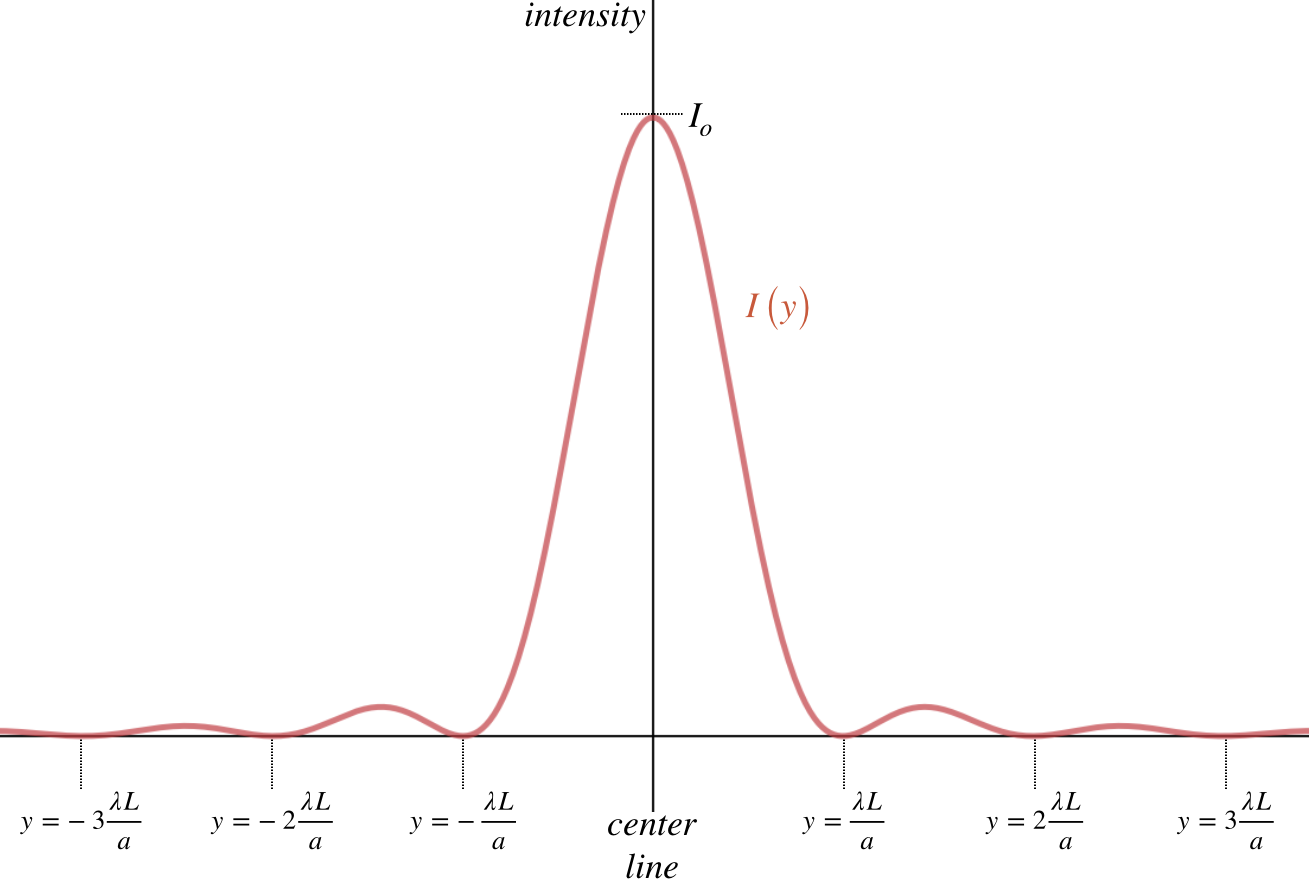
Let's point out a few of the more prominent features of this intensity pattern.

• The dark fringes are regularly spaced, in exactly the manner described by Equation 3.4.3 (note: \(\sin\theta\approx \frac{y}{L}\)).
• The central bright fringe has an intensity significantly greater than the other bright fringes, more that 20 times greater than the first order peak.
• Using calculus to find the placement of the non-central maxima reveals that they are not quite evenly-spaced – they do not fall halfway between the dark fringes.

We have assumed for simplicity the geometry of a long rectangular slit. If we were instead shining the light through a circular hole, this pattern would occur in every direction of two dimensions, resulting in concentric bright and dark circles, rather than fringes.

Example \(\PageIndex{1}\)

You are on a sunny Hawaiian beach, trying to relax after a grueling quarter of Physics 9B. You would like to recline in your beach chair with your feet in the water, but don’t want to get crushed by shore break while you snooze. About 100 meters off shore, you see an exposed reef that acts as a breakwater, but there is a gap in it, and waves (whose crests are parallel to the shore) are coming through that gap. While watching the waves, you see a surfer paddle out through the gap, and you use the perspective this event affords you to estimate that the gap is 25 meters wide (the diagram below is not to scale). You time a wave as it comes from the reef, estimating that it takes about 2 minutes for a wave to get to the shore from the gap, and the waves hit the shore roughly every 7 seconds. Starting from the point on the beach directly in line with the center of the gap, roughly how many paces (each pace being 1 meter in length) must you walk along the beach so that you can plant your beach chair and get the minimum wave intensity?

Solution

This is a problem in single-slit diffraction, where we are searching for the first “dark fringe” (place where destructive interference occurs). We can use Equation 3.4.3 for finding the angular deviation from the center line for a single slit, but it requires the wavelength of the wave as well as the slit gap. We have the latter, but we need to calculate the former. We can determine the wave speed and we are given the period, so:

\[\lambda=vT = \left(\dfrac{100m}{120s}\right)\left(7s\right) = 5.83m \nonumber\]

Now we can plug this wavelength into Equation 3.4.3 to find the angle of the first dark fringe:

\[\sin\theta = \dfrac{\lambda}{a}\;\;\;\Rightarrow\;\;\; \theta = \sin^{-1}\left(\dfrac{5.83m}{25m}\right) = 13.5^o \nonumber\]

The distance from the gap to the shoreline and the angle are known, so we can determine how far along the shore the dark fringe hits:

\[y = x\tan\theta = \left(100m\right)\tan13.5^o = 24m \nonumber\]

So you need to walk 24 paces.

You might be tempted to use the “small angle” equation to solve this more directly, and in fact the angle is quite small. But we have defined our measurement limits in terms of paces, and using the small angle formula we end up with an answer of 23 paces, so while the approximation is very good (it is only off by less than 5%), even our rather coarse measurement scheme notices the difference. [Okay, so "notice" might be too strong a word, as the wave intensity one pace from a minimum and 23 paces from the maximum is not going to be significant.]

 

Including Gap Size for Double Slits

Our analysis of double slits assumed that the slits were very thin, creating point sources. But in the real world, these slits must have finite gap widths (if the widths get too small, too little light gets through to see anything!). So how can we incorporate our result for single slit interference into what we found for double-slit interference? The easiest way to see the answer is to think of the single slit effect as putting limits on the light that comes through. If the light that would reach the screen in the absence of the single slit is a plane wave, then these limits just consist of the single slit intensity pattern (square of the sinc function). If the light destined to reach the screen is instead a double-slit intensity pattern, then the effect of the single slit is to squeeze down the bright peaks (reduce the brightness) so that they conform to the "envelope" of the single slit pattern. That is, the whole intensity pattern of the double-slit becomes the "\(I_o\)" for the single slit pattern. Mathematically, this is equivalent to multiplying the intensity functions:

\[\left. \begin{array}{l} I_\text{double slit}=I_o\cos^2\left(\dfrac{\Delta\Phi}{2}\right) &&\Delta\Phi = \dfrac{2\pi}{\lambda}d\sin\theta \\ I_\text{single slit} = I_o\left[\dfrac{\sin\alpha}{\alpha}\right]^2 && \alpha = \dfrac{\pi a}{\lambda}\sin\theta \end{array} \right\}\;\;\;\Rightarrow\;\;\; I_\text{both} = I_o\cos^2\left(\dfrac{\Delta\Phi}{2}\right)\left[\dfrac{\sin\alpha}{\alpha}\right]^2 \]

Figure 3.4.4 - Intensity Pattern for Double Slit with Finite Gap Widths

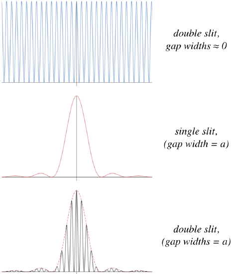
How does this actually appear to someone viewing it on the screen? The usual double-slit pattern is there, but the fringes are not all equally-bright. The center fringes are very bright, and it quickly tapers off. The single slit pattern is apparent in the brightness of the double-slit fringes. Notice, by the way, that we have assumed here that the slit separation is larger than the gap widths. This is apparent from the fact that the distance between dark fringes for the double slit is much smaller than it is for the single slit, and the separations are inversely-proportional to the slit separation \(d\) for the double slit, and inversely-proportional to the gap width \(a\) for the single slit.

Example \(\PageIndex{2}\)

Light is shone through a double slit apparatus whose slit gaps are wide enough to also exhibit single slit interference. The slit spacing for this apparatus is 4 times as great as the gap sizes. How many bright fringes from the double slit pattern appear within the central maximum of the single slit pattern (i.e. between the first order dark fringes)?

Solution

We are given that \(d = 4a\), so comparing the bright fringe equation for the double-slit (Equation 3.2.3) with the dark fringe equation of the single-slit (Equation 3.4.3), we see that the \(4^{th}\)-order bright fringe of the former coincides with the \(1^{st}\) dark fringe of the latter:

\[\left. \begin{array}{l} \text{double-slit bright fringes:} && m_\text{double-slit}\;\lambda = d\sin\theta \\ \text{single-slit dark fringes:} && m_\text{single-slit}\;\lambda = a\sin\theta \\ \text{given:} && d=4a \end{array} \right\} \;\;\;\Rightarrow\;\;\; m_\text{double-slit} = 4 m_\text{single-slit} \nonumber\]

This means that the \(4^{th}\)-order double-slit bright fringe won’t appear, as the destructive interference of the single slit will wipe it away. The central bright fringe and the three fringes (on each side) lie between these two endpoints. This makes a total 7 double-slit bright fringes within the central single-slit maximum.

Diffraction for an "Inverse Slit"

We can use our knowledge of waves to determine the light pattern we will see when the incoming plane wave diffracts around a thin barrier. Imagine starting with a plane barrier, out of which we cut a tiny sliver. Described above is what we see if coherent light is shone through the opening we have created in the barrier, but what if we shine the same light on just the sliver? That is, instead of only allowing light to pass through a thin space, we let the light pass everywhere except the thin space.

Imagine a tight laser beam in three different situations: First, it goes straight to the screen unimpeded. As with all laser beams, it spreads very little during its journey. Second, it encounters a thin slit that is a little bit smaller than the width of the beam. Naturally a single-slit diffraction pattern appears on the screen. And third, the beam encounters only a sliver that has the same dimensions as the single slit, so that the outer edges of the beam go past the edges of the sliver. Our question is what happens in this third case.

Figure 3.4.5 - Three Laser Beam Results

If the light from the second case was allowed to superpose with the light from the third case, it should be pretty clear that the result will be the first case. But for the second case, some light lands outside the beam's confines (thanks to diffraction), which means that for the superposition to occur, the third case must also send light to those outer regions with exactly the same amplitudes as the slit, though the light from the sliver must be \(\pi\) radians out of phase with the light from the slit. But if the sliver is by itself, the light it sends outside the beam region doesn't cancel with anything, which means it shows up on the screen. The end result is that the interference pattern outside the beam region must be the same for the sliver as it was for the slit.

What about the central bright fringe? For a single slit, the central maximum is not as bright as the unimpeded beam (because some of the light energy is diverted by diffraction). For the superposition to apply, this means that the region directly behind the sliver must also be illuminated. The relative brightness of the central maximum with the outer fringes may be different for the slit and the sliver, but the fringe spacings are the same in both cases, giving essentially the same diffraction patterns for both cases. This phenomenon is known as Babinet's principle.