
5.8: Special Processes
- Page ID
- 18475

Analyzing Special Processes
Next we will discuss some special processes, not only because they are themselves important, but because they are highly instructive. In this discussion, we will emphasize several aspects of each case:
- a physical picture of what is happening, using a gas trapped in a container with a moveable piston
- a schematic representation of what is happening with regard to heat transfer and work done
- an accounting of the fates of the various thermodynamic variables over the course of the process
- relationships between thermodynamic variables in the process due to state equations and the first law
- a \(PV\) diagram of the process
One must keep in mind that all of these processes are assumed to be quasi-static, which means that when arrows indicate heat transfer or work performed, this occurs due to an infinitesimal imbalance.
By “special processes,” we simply mean processes that eliminate from consideration one (or more) of the thermodynamic variables we have discussed so far. These variables include, volume, pressure, temperature, internal energy, heat, and work (particle number is already eliminated for every case, since we have decided to always hold it constant).
Isochoric Process
A process that involves no change in volume is called isochoric. With no change in volume, \(dV=0\), there can be no work done on or by the gas, which means that the only exchange of energy possible is through heat transfer, giving one of two physical situations, both including a pegged piston, and one with heat entering and the other with heat leaving.
Figure 5.8.1 – Isochoric Processes – Physical Picture
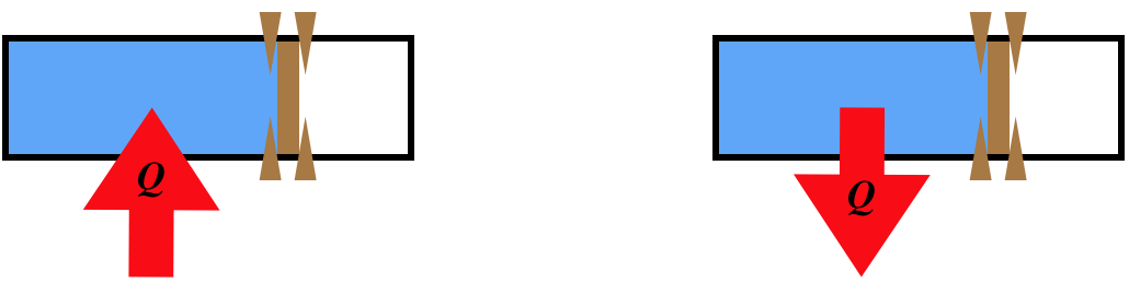
Having already determined what happens with the non-state variables of heat and work in these processes, let's do an accounting of the changes that occur in the state variables for an ideal gas. We will consider the case of heat energy entering the system – the changes that occur for the case when the system is losing heat should be obvious once this case is understood.
We already know that the volume doesn't change:
\[\Delta V = 0\]
With no work done, the first law requires that all of the internal energy change is due to heat transfer, and since the internal energy is proportional to the temperature, we get:
\[\Delta U=Q \;\;\; \Rightarrow \;\;\; \Delta U>0\;\; and \;\; \Delta T>0\]
What about the pressure? For this we can use the ideal gas law. We know that the temperature is increasing while the volume (and particle number) remains fixed, so the pressure goes up:
\[PV=nRT \;\;\;\Rightarrow\;\;\; \Delta P = \Delta \left(\dfrac{nRT}{V}\right) = \left(\dfrac{nR}{V}\right)\Delta T >0\]
Every process results in its own unique relationship between the non-state variables (work and heat) and changes in the state variables, and in this case we have:
\[\begin{array}{l} monatomic: && Q = \Delta U && = && \dfrac{3}{2}nR\Delta T && = && \dfrac{3}{2}\left(\Delta P\right) V \\ diatomic\;(no\;vibration\;mode): && Q = \Delta U && = && \dfrac{5}{2}nR\Delta T && = && \dfrac{5}{2}\left(\Delta P\right)V \\ general: && Q = \Delta U && = && nC_V\Delta T && = && \dfrac{C_V}{R}\left(\Delta P\right) V\;, \end{array}\]
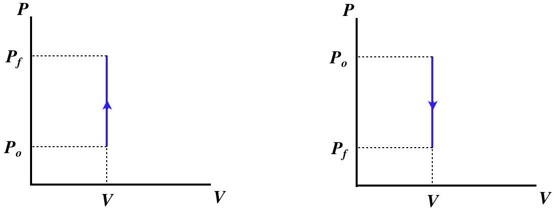
where \(C_V\) is given by Equation 5.6.7. The PV diagrams for these processes confirms that the work done (the area under the curve) is zero:
Figure 5.8.2 – Isochoric Processes – PV Diagram
A curve for an isochoric process is called an isochor.
Isobaric Process
A process that involves no change in pressure is called isobaric. We cannot draw a simple conclusion about work as we did in the isochoric case, because in this case the piston is free to move. However, we can use the ideal gas law and the first law to determine the physical picture. Let's take the case where the volume expands at constant pressure. We find from the ideal gas law that this requires the internal energy to go up:
\[\left. \begin{array}{l} P=constant \\ PV=nRT \\ \Delta V>0 \end{array} \right\} \;\;\; \Rightarrow \;\;\; \Delta T > 0 \;\;\; \Rightarrow \;\;\; \Delta U > 0\]
Now applying the first law and noting that the work done to expand the volume is positive, we find:
\[\left. \begin{array}{l} \Delta U = Q - W \\ W>0 \\ \Delta U > 0 \end{array} \right\} \;\;\; \Rightarrow \;\;\; Q>0\]
Therefore for an isobaric expansion of an ideal gas, heat must pass into the system. All of this can of course work in reverse as well, so we have the following physical pictures:
Figure 5.8.3 – Isobaric Processes – Physical Picture

In determining this physical picture, we determined all the state variable changes that occur. All that is left is to relate the heat and work to the state variable changes. The work we can compute easily from the pressure and volume, since the pressure is constant:
\[W=\int\limits_{V_o}^{V_f}PdV = P\int\limits_{V_o}^{V_f}dV = P\Delta V\]
From the ideal gas law, we can also write this in terms of the temperature change:
We already have the relationship between the internal energy and temperature, so we can use the first law to write the relationship between the heat transferred and the change in state variables:
where again \(C_V\) is given by Equation 5.6.7. The PV diagrams for these processes are simple enough – constant pressure translates to a horizontal graph:
Figure 5.8.4 – Isobaric Processes – PV Diagram
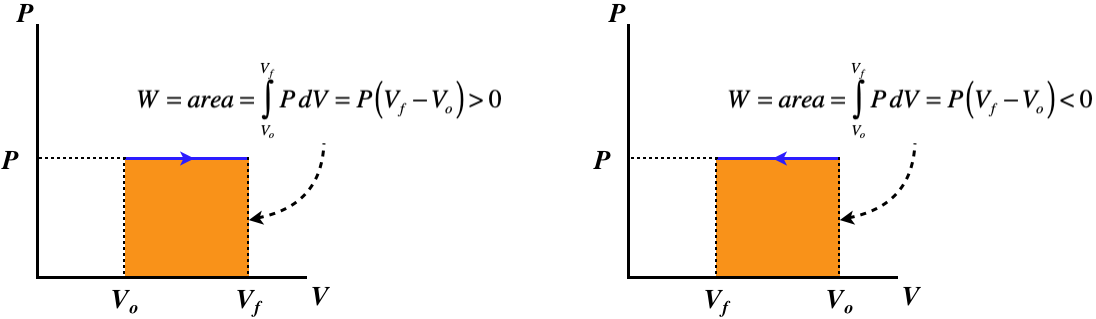
A curve for an isobaric process is called an isobar.
Heat Capacity
In Section 5.6, we noted that the relationship between the heat added and the change in temperature defines the molar heat capacity. It was noted then that this quantity is not a fixed constant for a given gas, but instead depends upon the process. With the the first law of thermodynamics and the fixed relationship between internal energy and temperature, we have:
\[Q = \Delta U + W = nC_V\Delta T + W = nC\Delta T\]
The molar heat capacity \(C\) is defined from the process by determining how the work done in that process is related to the temperature change. The quantity \(nR\Delta T\) has units of energy, and is scaled for \(n\) moles of a gas, so if we measure the work done by a process as \(\alpha\) of these units, we can write the heat transferred in terms of the temperature change as:
\[W=\alpha \left(nR\Delta T\right) \;\;\;\Rightarrow\;\;\; Q = nC_V\Delta T + n\alpha R\Delta T = n\left(C_V+\alpha R\right) \Delta T \;\;\;\Rightarrow\;\;\; C = C_V+\alpha R\]
So if we can determine the value of \(\alpha\) for the process, we can compute the molar heat capacity. Since heat capacity is a measure of how much heat can be added to a system for a given temperature increase, it makes sense that if energy comes out of the system in the form of work, then more heat can be transferred for the same temperature change than if the work did not remove energy.
We have now seen two special processes, and we have the values of \(\alpha\) for both of them. For the isochoric process, there is zero work done, so \(\alpha=0\), giving simply \(C = C_V\). Now we see why we originally appended the "\(V\)" in the subscript – because this constant happens to equal the molar heat capacity at constant volume. For the isobaric process, we got a different value for \(\alpha\). From Equation 5.8.8, we see that for this process \(\alpha = 1\), which gives us the molar heat capacity at constant pressure:
\[C_P = C_V + R\]
Notice that this takes into account the number of modes, because that information is contained in \(C_V\). So for monatomic ideal gases, \(C_P=\frac{5}{2}R\), for diatomic ideal gases, \(C_P=\frac{7}{2}R\), and so on.
Example \(\PageIndex{1}\)
One mole of a diatomic ideal gas is confined to a piston and undergoes a quasi-static process where \(\frac{1}{4}th\) of the added heat is converted into work. Find the molar heat capacity for this process.
- Solution
-
Plugging \(W=\frac{1}{4}Q\) into the first law gives:
\[\Delta U = Q - W = Q - \frac{1}{4}Q \;\;\;\Rightarrow\;\;\; Q=\frac{4}{3}\Delta U = \frac{4}{3}\left(nC_V\Delta T\right) \;\;\;\Rightarrow\;\;\; C = \frac{4}{3}C_V\nonumber\]
Now we plug in for the constant \(C_V\) for a diatomic ideal gas (for which, as always, we assume that the vibrational modes are frozen out) to get our answer:
\[C_V = \frac{1}{2} R \times \left( number \; of \; modes \right) = \frac{5}{2} R \;\;\; \Rightarrow \;\;\; C = \frac{10}{3} R \nonumber \]
Gases can be mixtures of varieties (monatomic, diatomic without vibration, etc.), and it can be cumbersome computing the contributions of modes by each, so a more efficient method has been devised to characterize gases in the form of a constant \(\gamma\), defined as:
\[\gamma \equiv \dfrac{C_P}{C_V} = 1+\dfrac{R}{C_V}\]
In the cases where the gases are of a single type, this constant tells us exactly what type it is:
\[\begin{array}{l} monatomic: && \gamma=\dfrac{5}{3} \\ diatomic: && \gamma=\dfrac{7}{5} \\ polyatomic: && \gamma=\dfrac{4}{3} \end{array}\]
When the gas is a mixture, this constant lands between these values. Note that \(\gamma\) drops in value as more modes become available.
Isothermal Process
A process that involves no change in temperature is called isothermal. In this case, a constant temperature means a constant internal energy, and from the first law we get that the heat transferred equals the work done:
\[T=constant \Rightarrow \;\;\; 0=\Delta U=Q - W \;\;\; \Rightarrow \;\;\; Q=W\]
From our sign conventions for \(Q\) and \(W\), we know that this means that if heat is entering the system, then the gas is doing work, and if heat is exiting the system, then work is being done on the gas. This gives the same basic physical picture as given above for the isobaric process, though the details are distinctly different, as is seen in the effects on the state variables. Let's consider the case of the expanding gas: The volume increases (\(\Delta V>0\)), and the temperature and internal energy remains constant (\(\Delta T=0\;,\;\;\Delta U=0\)), so from the ideal gas law, the pressure must be going down (\(\Delta P<0\)).
Next we want to write the work and heat in terms of the changes in state variables. Fortunately, these two quantities equal each other in this case, so if we compute one, we immediately have the other. We can compute the work done with the integral, because the constant temperature and ideal gas law enables us to write the pressure as a function of the volume:
There are a number of differences between this process and the others we saw before it:
- The natural logarithm function makes an appearance in the calculation of the heat or work from the state variables, and either the volumes or pressures can be used in the calculation.
- The relationship between heat or work and the state variables does not depend upon whether the gas is monatomic, diatomic, etc. This makes sense, because this process involves no change in the internal energy, so the number of modes available for energy distribution is irrelevant.
- The molar heat capacity is infinite, since any amount of heat can be added and the temperature never changes.
The PV curve is no longer so trivial:
Figure 5.8.5 – Isothermal Processes – PV Diagram
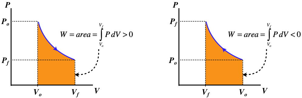
A curve for an isothermal process is called an isotherm.
Example \(\PageIndex{2}\)
The \(PV\) diagram below depicts two equilibrium states (“A” and “B”) of two moles of an ideal gas confined by a piston which both lie on the same isotherm. You are supplied with a meter stick and a thermometer, so you can determine the volume of the piston and the temperature of the gas at any stage. Suppose you take the system from state B to state A. You do this in two stages: First you compress the gas at a constant pressure to the final volume, then you raise the pressure to the final pressure with a fixed volume. You measure the two volumes to be \(V_A=0.130m^3\) and \(V_B=0.160m^3\), and before you start the compression, your thermometer measures the temperature of the gas to be \(T=292K\).

- Sketch this two-stage process (including an arrow to indicate the direction) on the diagram and use the sketch to compute the total work done on or by the gas (specify which) in joules.
- Find the total heat that enters or exits the system (specify which) during this two-stage process.
- Suppose you repeat this two-stage process with two different gases – \(He\) and \(N_2\). During the process, which gas will exhibit the greatest difference between its maximum and minimum internal energy, or will both be the same?
- Solution
-
a.
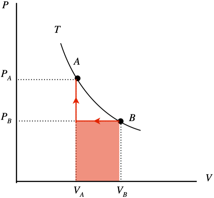
The work done during the second process is zero, so the total work done by the two processes is the shaded area shown under the curve. The process goes right-to-left, so the work done is negative, which means it is work done on the system:
\[W=P_B\left(V_A-V_B\right)\nonumber\]
The starting temperature \(T_B\) is known, as is the number of moles, and the volume so the starting pressure can be computed, giving us the work:
\[P_B = \dfrac{nRT_B}{V_B} = \dfrac{\left(2mol\right)\left(8.31\frac{J}{mol\;K}\right)\left(292K\right)}{0.160m^3} = 3.03\times 10^4 Pa \;\;\; \Rightarrow \;\;\; W=\left(3.03\times 10^4 Pa\right)\left(0.130m^3-0.160m^3\right) = -910J \nonumber\]
b. The system begins and ends with the same temperature, since both states are on the same isotherm. Therefore it begins and ends with the same internal energy, which means that all the energy that comes in as work goes out as heat: \(Q = -910J\).
c. In both cases the gases pass through the same pressures and volumes, which means they will exhibit the same temperatures throughout (they both satisfy the same ideal gas law). The internal energy, on the other hand, will be different for the two, since its relationship with the temperature is different. For the same temperature change \(\Delta T\), the gas with the higher heat capacity will experience the greater change in internal energy. Therefore \(N_2\) (which is diatomic and therefore has 5 modes per particle compared to 3 for monatomic He) exhibits the higher internal energy change.
Adiabatic Process
A process that involves no heat exchange is called adiabatic. Like the isochoric case, this makes the physical picture an easy one to describe. One difference that is added to the diagram is insulation of the container in the form of thicker walls, to represent the inability of heat to transfer into or out of the system.
Figure 5.8.6 – Adiabatic Processes – Physical Picture

The first law tells us immediately that the internal energy change is entirely caused by work done on or by the system:
\[\Delta U = Q - W = -W\]
In the case of the gas expanding, positive work is done, which means that \(\Delta U < 0\) and \(\Delta T < 0\). With volume increasing and temperature decreasing, the ideal gas law tells us that the pressure must be going down during this expansion. The relationship between the work and the change of state variables is easy to compute from its relationship to internal energy:
We see that the work done on or by the gas depends upon the type of gas. It therefore becomes useful to express the work done in terms of the constant \(\gamma\) for the gas. Plugging Equation 5.8.13 into Equation 5.8.18 gives:
\[W = \dfrac{1}{1-\gamma}\left(P_fV_f - P_oV_o\right) \]
Example \(\PageIndex{3}\)
Each of the four "special processes" involves its own unique graph on the \(PV\) diagram of the quasi-static process. The graph of the isochoric process is a vertical line (\(V=const\)); the graph of the isobaric process is a horizontal line (\(P=const\)); and the graph of the isothermal process is a hyperbola (\(P= \dfrac{const}{V}\)). Use the result for the work done in an adiabatic process to show that the graph of this process on the \(PV\) diagram is (\(P=const \;V^{-\gamma}\)).
- Solution
-
Plugging the function \(P = const\;V^{-\gamma}\) into the work integral does the job:
\[W = \int\limits_{V_o}^{V_f}PdV = const\;\int\limits_{V_o}^{V_f}V^{-\gamma}dV = const\; \left[\dfrac{V^{-\gamma+1}}{-\gamma+1}\right]_{V_o}^{V_f} = \dfrac{const}{1-\gamma}\; \left[V_f^{-\gamma+1} - V_o^{-\gamma+1}\right] = \dfrac{1}{1-\gamma}\; \left[const\;V_f^{-\gamma} V_f - const\;V_o^{-\gamma}V_o\right] = \dfrac{P_fV_f-P_oV_o}{1-\gamma}\nonumber\]
The graph for the \(PV\) diagram for an adiabatic process (called an adiabat) looks similar to that of an isotherm – the only difference is the magnitude of the exponent of the volume. In the example above, we showed that the graph is defined by:
\[adiabatic\;process:\;\;\;\;\; P = const\;V^{-\gamma} \]
The constant \(\gamma\) is always greater than 1 for any gas, so it is not difficult to show mathematically that for a single system, the adiabat that passes through a given point in the \(PV\) plane is steeper than the isotherm (defined by \(P = const\;V^{-1}\)) that passes through the same point. This makes sense, since one would expect that the pressure would drop faster as a gas expands when there is no heat entering the system.