7.2: Kepler's Laws

More than 20 years before Newton was born, a fellow named Johannes Kepler took a shot at explaining the orbits of the planets. He too posited that physical laws might be able to explain the motions, but didn’t possess the tools (mathematical and physical) at Newton’s disposal decades later (though admittedly, Newton did develop these tools for himself). Instead, what Kepler had were the remarkably detailed and accurate measurements of planetary motions made by an astronomer named Tycho Brahe, which he used to look for patterns in the motions. Amazingly, he found that the planets indeed moved with mathematical precision, and published his three laws of celestial motion, all of which are in exact accordance with the law of universal gravitation. While reading about his three laws, consider what a monumental accomplishment this was. Tycho Brahe's data detailed the motions of the planets as he viewed them from Earth (which itself is orbiting the sun).

Kepler’s First Law

Kepler's First Law: The paths of bodies trapped in orbits form closed ellipses, with the gravitating body at one of the foci.

The many elements of an ellipse and how an orbit fits into the picture are expressed in Figure 7.2.1.

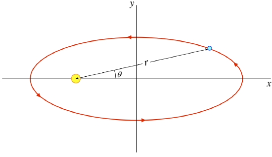
Figure 7.2.1 – Elliptical Orbit

There are many ways to describe such an orbit mathematically. A common way is to write the distance between the two bodies as a function of the angle that the line between them makes with the major (longer) axis:

Figure 7.2.2 – Polar Coordinate Description of Ellipse

The formula for the ellipse in these coordinates is:

\[ r\left(\theta\right)=\dfrac{a\left(1-e^2\right)}{1-e\cos\theta} \]

[Note: It is also possible to measure the angle in the opposite direction (with \(\theta=0\) corresponding to the perihelion), in which case the denominator is a sum rather than a difference.]

Circles are special cases of ellipses (eccentricity equal to zero), so naturally circular orbits are possible. Notice that if we plug in \(e=0\) above, we get the simple orbit equation \(r=a\). With a great deal of mathematics (first surmounted by Isaac Newton), one can can show that in fact this is a natural consequence of the inverse-square force law we already stated for gravitation. While we won't go quite so far as to perform this derivation, below we will make a closer examination of features of the ellipse (which we have expressed as a purely mathematical object here) in terms of physical quantities.

Kepler’s Second Law

Kepler's Second Law: An orbiting planet sweeps out equal areas in equal times during its orbit.

Kepler noticed that the planet moved faster when it was near the perihelion than when it was near the aphelion, and through painstaking examination of the data determined that in fact the amount of area the orbit sweeps out in a given period of time is the same everywhere in the orbit.

Figure 7.2.3 – Equal Areas in Equal Times

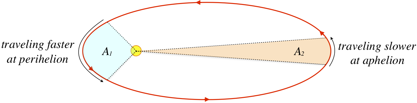
Note that while the diagram compares areas swept out through the perihelion and aphelion, the result applies to any part of the orbit – if we wait the same period of time, the area swept out will be the same: \(A_1=A_2\). We will soon look into the physical aspects of gravitational orbits that lead to this result, but again one can't help but marvel at what it must have taken to derive this remarkable discovery from the raw data.

Kepler’s Third Law

Kepler's Third Law: For every object orbiting the same gravitational source, the ratio of the cube of the semi-major axis of the orbital ellipse and the square of the orbital period is the same constant: \(\dfrac{a^3}{T^2} = constant\).

While the first law makes a general statement about all gravitational orbits, and the second law relates two different parts of a specific gravitational orbit, the third law gives a way of comparing different orbits of the same gravitating object (in Kepler's case, this gravitating object was the sun). Of the three laws, this one has the greatest practical value, because it means that even without knowing anything about the law of gravitation, one can make a prediction about one orbiting body based on observations of another orbiting body, if both are going around the same gravitating object. We will see what this mysterious constant is in terms of physical details, but to solve certain problems, knowing the actual value of the constant isn't necessary.

Example \(\PageIndex{1}\)

An astronomer notices that an asteroid is positioned such that the Earth is directly between it and the Sun. It has a roughly circular orbit (like the Earth), which is in the same plane and in the same direction as the Earth. This asteroid is far away from the Earth – about 8 times farther from the Earth than the distance separating the Earth and the Sun. These are all approximations, but about how long will this astronomer have to wait see these three bodies reach these same positions?

Solution

For a circular orbit, the semi-major axis of the orbit is simply the radius of the orbit, and since the asteroid and Earth are both orbiting the same gravitational source (the sun), then Kepler's third law results in the same constant for both:

\[ \dfrac{R_{earth}^3}{T_{earth}^2} = constant = \dfrac{R_{asteroid}^3}{T_{asteroid}^2} \;\;\; \Rightarrow \;\;\; T_{asteroid}=\left(\dfrac{R_{asteroid}}{R_{earth}}\right)^{\frac{3}{2}}T_{earth} \nonumber \]

The period of the Earth's orbit is exactly 1 year, and the asteroid is 9 times farther from the sun as the Earth, so the time it will take the asteroid to come back to the same spot will be:

\[ T_{asteroid} = 27years \nonumber \]

Of course, in 27 years, the Earth will also be in the spot where it started, so this is our answer.

Note that if the question asked for the time that elapses before the sun, Earth, and asteroid are all aligned again (which is different from reaching their original positions), the answer is different: When they realign for the first time, the Earth will have completed one orbit plus a bit more, while the asteroid will have completed a fraction of an orbit. Let's call the angle that the asteroid moves through in that first year \(\Delta \theta\). The Earth catches up to it after a full revolution, so the angle the Earth moves through is:

\[ \theta_{earth} = 2\pi + \Delta \theta \nonumber \]

The Earth is moving 27 times as fast as the asteroid, so in this equal time frame the Earth has moved through an angle 27 times as great as the asteroid, which gives:

\[ 2\pi + \Delta \theta = 27\Delta \theta \;\;\; \Rightarrow \;\;\; \Delta \theta = \dfrac{2 \pi}{26} \nonumber \]

That is, the asteroid completes 1/26th of its orbit at the point when the Earth catches up to it. The asteroid's orbit takes 27 years, so the first alignment occurs at:

\[\Delta T = \dfrac{27years}{26} = 1 year, 14 days \nonumber \]

A nice application of Kepler’s 3rd law involves man-made satellites that orbit the Earth. Telecommunications satellites we like to remain at a single position in the sky, so that we don’t have to turn our satellite dishes to find them – we just point them in the right direction and leave it. To accomplish this, we need two things: The satellite has to be directly above the equator, and it has to be orbiting the Earth in the same direction that the Earth is rotating, with an orbital period of exactly 1 day. This is known as a geostationary orbit. We can use Kepler’s 3rd law to determine how high off the Earth’s surface this satellite needs to be.

Reconciling Kepler’s Laws with Universal Gravitation

There are a couple of things we can say about the physics of gravitational orbits. First, gravity is a conservative force, which means that the mechanical energy of the system is conserved. We don't yet know how to describe the potential energy due to the gravitational force (hopefully it is clear that our old "\(U\left(y\right) = mgy + U_o\)" treatment is no longer adequate, since this results in a constant force), but we will look at this in Section 7.3. The point is that the mechanical energy is a "constant of the motion," which we can use, for example, to describe the speed of the orbiting body as a function of the distance from the gravitational source.

Consider the Earth + sun system. The fraction of this system's mass that belongs to the Earth is about \(3 \times 10^{-6}\), which means that the distance from the center of the sun to the center of mass of the system is this fraction multiplied by the (on average) 93 million miles separating the two bodies. The distance from the center of the sun to the center of mass of the system is therefore:

\[ r_{cm} = \left(3 \times 10^{-6}\right)\left(93 \times 10^6\;miles\right) = 279 \; miles\]

The radius of the sun is about 432,000 miles, so the center of mass of the system lies less than one tenth of one percent of the sun's radius from the sun's center. It's therefore a pretty good approximation to treat the center of the sun as a fixed point. [Note: Even the center of mass of the Jupiter + sun system barely lies outside the sun's radius, even though Jupiter is much more massive than Earth, and is much farther away.] The gravitational force is directed at this fixed point, so it constitutes a central force. As we found in Section 6.2, central forces have the property of conserving the angular momentum of the system (since they produce no torque). We therefore conclude that like the mechanical energy, the angular momentum of an orbiting body is also a constant of the motion, when the gravitating body is significantly more massive than the orbiting body. [Note: The angular momentum of the whole system is always conserved, even when the two masses are comparable, but in that case we can't treat one object as orbiting another stationary one, which means we have to consider the motion of both objects, complicating our picture.]

Kepler's First Law

Showing that elliptical orbits are a direct result of the law of universal gravitation is a mathematical exercise that is somewhat beyond the scope of this work. While this derivation could nevertheless be included here, the value of doing so is minimal, and will therefore be left for the reader to explore in an upper-division treatment of classical mechanics. Instead, we will look at only small – but very instructive – aspects of Kepler's first law.

Never mind that we have no reason to expect that orbits will be elliptical... Why would we even expect them to be closed? That is, it certainly isn't clear that when the polar angle \(\theta\) changes by \(2\pi\), that the orbiting body's distance from the gravitating body will be the same. It turns out, however, that this element of gravitational orbits is not hard to demonstrate. Start by applying Newton's second law to the orbiting body on which a net force due to gravity is acting:

\[ m\dfrac{d\overrightarrow v}{dt} = -\dfrac{GMm}{r^2} \widehat r \]

We can rewrite this in terms of how the velocity changes with the angle \(\theta\) by using the chain rule:

\[ m\dfrac{d\overrightarrow v}{d\theta}\dfrac{d\theta}{dt} = -\dfrac{GMm}{r^2} \widehat r \]

The angular momentum of the orbiting body can be written in terms of its mass, its angular velocity \(\omega = \dfrac{d\theta}{dt}\), and its distance from the fixed point:

\[ L = mr^2\omega \]

This angular momentum is a constant of the motion (i.e. it is conserved throughout the orbit), so we find that the rate at which the velocity vector changes with respect to \(\theta\) is a vector with a constant magnitude:

\[ \dfrac{d\overrightarrow v}{d\theta} = -\dfrac{GMm}{L} \widehat r \]

We can write the position unit vector in terms of the angle relative to a cartesian coordinate system, as we did in Equation 1.6.11:

\[ \dfrac{d\overrightarrow v}{d\theta} = -\dfrac{GMm}{L} \left( \cos \theta \; \widehat i \ + \sin \theta \; \widehat j \right) \]

Integrating over the angle gives the velocity vector as a function of \(\theta\) (and an undetermined constant of integration \(\overrightarrow v_o\)):

\[ \overrightarrow v\left(\theta\right) = -\dfrac{GMm}{L} \left( \sin \theta \; \widehat i - \cos \theta \; \widehat j \right) + \overrightarrow v_o \]

From this result we can conclude that the magnitude and direction of the velocity return to the same value every time \(\theta\) changes by \(2\pi\). This means that the kinetic energy returns to its same value periodically as well. But the mechanical energy of this system is conserved, so the potential energy also returns to its value with the same periodicity. But (as we will see in the next section), the potential energy is defined by the separation of the two masses, so this separation also returns every time \(\theta\) changes by \(2\pi\). Well, if every time the angle changes by \(2\pi\) the orbiting body is the same distance away from the gravitating body, is moving at the same speed, and is moving in the same direction, then clearly its motion is being repeated – the orbit is closed.

Notice that if dependence on \(r\) in the law of gravitation was anything other than inverse-square, then the \(r\)'s would not cancel as they did in reaching Equation 7.2.6 (the angular momentum would still be the same constant of the motion, as the force would still be central), which would give an equation for the velocity that depends on both \(r\) and \(\theta\). This ruins the argument above, and the orbit would not be closed.

Digression: Orbits Are Not Quite Closed After All

As amazing as Newton's accomplishment was with his theory of gravity, roughly 230 years later a fellow named Albert Einstein provided an improved theory, called the General Theory of Relativity. It had been known for some time that observations of the orbit of Mercury indicated that its orbit was in fact not closed. For a long time it was thought that the discrepancy was the result of an unseen planet or other gravitating body that was pulling Mercury off course, but Einstein's theory showed that the inverse-square theory of Newton, while a very good approximation, is not quite right, and his new theory predicted Mercury's motion perfectly.

While we are skipping the mathematics detailing how we get to the equation of the ellipse, we can still extract some information from Equation 7.2.8 that will be useful to us later. To simplify the discussion that follows, we will assume that we already know that the elliptical orbit is the result.

We haven't yet defined the orientation of the \(\left(x,y\right)\) coordinate system used in Equation 7.2.8 – so far we have only required that the origin be at the gravitating body. Let's choose the \(x\)-axis to lie along the major axis such that the point of maximum separation (aphelion) lies on the positive side of the \(x\)-axis (giving us Figure 7.2.2). With these axes, it is clear that at the point \(\theta = 0\), the velocity of the orbiting body is in the \(+\widehat j\) direction. Looking at Equation 7.2.8, we see that this means that the constant vector \(\overrightarrow v_o\) must point parallel to the minor axis, otherwise it would give the body a component of velocity along the \(x\) direction. But which way does this constant vector point, \(+\widehat j\) or \(-\widehat j\)?

Consider the velocity of the orbiting body at the perihelion (\(\theta = \pi\)). In this case, the object is now moving in the \(-\widehat j\) direction, but because it is closer to the reference point at the gravitating body, it must be moving faster to conserve angular momentum. For the constant vector \(\overrightarrow v_o\) to make the orbiting body faster at (\(\theta = \pi\)) than at (\(\theta = 0\)), we must have:

\[\overrightarrow v_o = v_o \left(-\widehat j \right) \;\;\; \Rightarrow \;\;\; \left\{ \begin{array}{l} \theta = 0 & \left(aphelion\right) & v_{min} = \dfrac{GMm}{L} - v_o \\ \theta = \pi & \left(perihelion\right) & v_{max} = \dfrac{GMm}{L} + v_o \end{array} \right. \]

We can relate the maximum and minimum speeds of the orbit using angular momentum conservation. Looking at Figure 7.2.1, we see that the value of \(r_\bot\) for the aphelion is: \(a+ea = a\left(1+e\right)\). At the perihelion: \(r_\bot = a\left(1-e\right)\). Setting equal the angular momenta at these two positions in the orbit gives:

\[ L_{aphelion} = L_{perihelion} \;\;\; \Rightarrow \;\;\; mv_{min}\left[a\left(1+e\right)\right] = mv_{max}\left[a\left(1-e\right)\right] \;\;\; \Rightarrow \;\;\; v_{min} = v_{max}\left(\dfrac{1-e}{1+e}\right) \]

Using this result and Equations 7.2.9, we can eliminate the troublesome \(v_o\), and get:

\[ \begin{array}{l} v_{max} = \left(1+e\right)\dfrac{GMm}{L} \\ v_{min} = \left(1-e\right)\dfrac{GMm}{L} \end{array} \]

It will also be useful to have an expression for the angular momentum in terms of the masses, eccentricity, and major axis. To get this, multiply the first of the Equations 7.2.11 by the orbiting body's mass and \(r_\bot\) [for \(v_{max}\) this is: \(a\left(1-e\right)\)] to get:

\[ L = mv_{max}r_\bot = m\left[ \left(1+e\right)\dfrac{GMm}{L}\right] \left[ a\left(1-e\right) \right] \;\;\; \Rightarrow \;\;\; L^2= a\left(1-e^2\right)GMm^2 \]

Putting this back into Equation 7.2.1 simplifies it a bit in terms of physical constants, putting it in a form that will be useful later:

\[ r\left(\theta\right)=\left(\dfrac{L^2}{GMm^2}\right)\dfrac{1}{1-e\cos\theta} \]

One last thing to note before moving on to Kepler's second law. Looking at Equation 7.2.8, we see that if \(v_o\) happens to equal zero, then the velocity vector has a constant magnitude, and its direction is always perpendicular to \(\widehat r\) (which can be confirmed quickly by performing a dot product). So a non-zero constant of integration is responsible for making an otherwise circular orbit eccentric.

Example \(\PageIndex{2}\)

Show that the distance of closest approach (the perihelion distance) is given by:

\[ r_{min} = \dfrac{L^2}{GMm^2}\left(\dfrac{1}{1+e}\right) \nonumber \]

Do this in two different ways:

1. Using calculus and Equation 7.2.13. [Note: There are two angles that result in extrema, but only one gives a minimum.]
2. Using the equation for angular momentum at \(r_{min}\) and one of the Equations 7.2.11.

Solution

a. We seek the minimum value of \(r\left(\theta\right)\), so we start by finding the value of \(\theta\) where this minimum occurs:

\[ 0 = \left(\dfrac{L^2}{GMm^2}\right)\dfrac{d}{d\theta}\left(\dfrac{1}{1-e\cos\theta}\right) \;\;\; \Rightarrow \;\;\; 0 = \dfrac{\sin\theta}{1-e\cos\theta} \;\;\; \Rightarrow \;\;\; \theta = 0 \;\; or\;\; \pi \nonumber \]

Note that \(\theta = 0\) minimizes the denominator, so it gives a maximum for \(r\), not a minimum. On the other hand, \(\theta = \pi\) maximizes the denominator, and therefore gives a minimum. This result makes sense when we look at how \(\theta\) is defined in Figure 7.2.2. Plugging \(\theta = \pi\) into Equation 7.2.13 gives the desired answer.

b. The angular momentum at the point closest approach will involve the maximum speed, since it is conserved throughout the orbit, so using the expression for the maximum speed in Equations 7.2.11 we get:

\[ L = mv_{max} r_{min} \;\;\; \Rightarrow \;\;\; r_{min} = \dfrac{L}{mv_{max}} = \dfrac{L}{m\left( \left(1+e\right)\dfrac{GMm}{L}\right)} = \dfrac{L^2}{GMm^2}\left(\dfrac{1}{1+e}\right) \nonumber\]

Kepler's Second Law

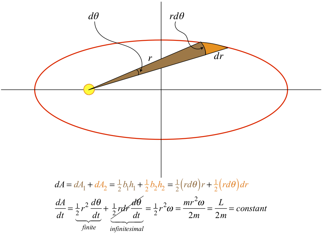
We look next at Kepler's equal-areas-swept-out-in-equal-times law. The geometry of measuring areas swept out of ellipses is impossibly difficult to do mathematically, but an infinitesimal amount of area swept out in an infinitesimal time period is something we can do. Figure 7.2.4 shows how we can mathematically describe the area swept out in an infinitesimal period of time. The amount swept out can be broken into two triangles. Okay, so the sides of the triangles are curved, but when the curves are infinitesimal in length, the amount they differ from straight lines is insignificant. The area of the two triangles are color-coded in the diagram. We notice that while both have infinitesimal areas, the orange triangle includes a product of two infinitesimal quantities. When the area is then divided by a small time span and the limit is taken as the time span goes to zero, the ratio of \(d\theta\) and \(dt\) approaches a finite value (specifically, the angular velocity \(\omega\) at that moment in time), but in the second term there is still another infinitesimal \(dr\) that goes to zero in the limit. In other words, the orange triangle contributes nothing to the area swept out in the infinitesimal time span \(dt\). With a little mathematical manipulation, we see that the rate at which area is swept out is the angular momentum of the orbiting body divided by twice its mass. We know that both the angular momentum and the mass remain constant for the orbit, so the rate at which area is swept out also remains constant. Kepler's second law is equivalent to angular momentum conservation.

Figure 7.2.4 – Kepler's Second Law Expresses Angular Momentum Conservation

Kepler's Third Law

It is quite straightforward to show that Kepler's third law holds for circular orbits, so let's do that first. The speed is constant for the entire orbit, it equals the circumference of the orbit divided by the time it takes for a full orbit:

\[ v = \dfrac{2\pi R}{T} \]

We can use the fact that the gravitational force is causing centripetal acceleration to get the following expression for the square of the constant speed of the orbiting body:

\[ \dfrac{GMm}{R^2}=m\dfrac{v^2}{R} \;\;\; \Rightarrow \;\;\; v^2 = \dfrac{GM}{R} \]

Plugging Equation 7.2.14 into Equation 7.2.15 and doing some algebra gives Kepler's third law, with the semi-major axis equaling the radius of the circular orbit (zero eccentricity):

\[ \left( \dfrac{2\pi R}{T}\right)^2 = \dfrac{GM}{R} \;\;\; \Rightarrow \;\;\; \dfrac{R^3}{T^2}= \dfrac{GM}{4\pi^2} = constant \]

This gives us not only that the ratio is a constant, but specifically what the constant is. As we can now confirm, this constant depends only upon the mass of the gravitating body.

It's quite remarkable that this law holds equally well for elliptical orbits, where \(R\) is replaced by \(a\). We can show this by starting with a result we found from Kepler's second law. The rate at which area is swept out is constant, so the total area of the ellipse is this rate multiplied by the time of a full orbit. Reviewing our conic sections, we plug in the area of an ellipse, and get:

\[ area\;of\;ellipse = \pi \; ab = \dfrac{dA}{dt} T = \dfrac{L}{2m} T \]

The quantity \(b\) is the length of the semi-minor axis, which is related to the length of the semi-major axis in terms of the eccentricity:

\[ b^2 = a^2\left(1-e^2\right) \]

Squaring Equation 7.2.17 and eliminating \(b^2\) using Equation 7.2.18 gives us:

\[ \pi^2 a^4 \left(1-e^2\right) = \dfrac{L^2T^2}{4m^2}\]

We had the good foresight to derive Equation 7.2.12, so plugging \(L^2\) from that equation into Equation 7.2.19 gives us our answer:

\[ \pi^2 a^4 \left(1-e^2\right) = \left[a \left(1-e^2\right) GMm^2 \right] \dfrac{T^2}{4m^2} \;\;\; \Rightarrow \;\;\; \dfrac{a^3}{T^2}= \dfrac{GM}{4\pi^2} \]

Example \(\PageIndex{3}\)

Attractive central forces that are not inverse-square do not produce closed orbits except when the orbit happens to be circular. Whenever there is a closed orbit, a result like Kepler's third law (which relates the orbit period to the radius of the circular orbit) will be the result. Derive the effective Kepler third law for an attractive central force that varies as the inverse-cube of the separation.

Solution

Following the process used above for a gravitational circular orbit, we get:

\[ \left. \begin{array}{l} \dfrac{k}{R^3}=m\dfrac{v^2}{R} \\ v = \dfrac{2\pi R}{T} \end{array} \right\} \;\;\; \Rightarrow \;\;\; \boxed{\dfrac{R^4}{T^2} = \dfrac{k}{4\pi^2m} = constant} \nonumber \]