27: Cosmic Microwave Background Anisotropies

Introduction

The plasma that existed from the first fractions of a second of the Big Bang until it transitioned to a neutral gas 380,000 years later is a beautiful gift of nature. Gently disturbed away from equilibrium by mysterious, very early-universe processes, the plasma is an unusually simple, natural dynamical system. Due to its simplicity, we can calculate the evolution of these disturbances with high accuracy and use these calculations to predict observable consequences. The agreement between our predictions and precision observations is extraordinary, allowing us a high degree of confidence that we understand in detail events that were transpiring 14 billion years ago, throughout the cosmos, as far away as the edge of the observable universe.

The simplicity of this system is perhaps best understood in contrast to other natural systems. Naturally occurring phenomena are usually too complicated to understand fully from first principles. We know the underlying physics, but the equations are really complicated to solve, and we’d need an absurd amount of data to narrow down from the set of all possible solutions of the equations, to the one that is actually being realized with the phenomenon in question. Examples of complicated phenomena are supernova explosions, earthquakes, and human behavior. We think we know the underlying physics at play, but getting from there to predictions for observations is extremely difficult, if not impossible. 

Usually, to observe a system for which we can make predictions, we need to carefully construct the system ourselves. We call such carefully constructed scenarios, ‘experiments.’ Although the exception rather than the rule, there are examples of naturally occurring systems that are amenable to our understanding. The solar system is such a naturally occurring system, with its simplicity arising from the fact that gravity is the dominantly important force, and the high accuracy of the simplifying approximation of the planets and stars as point masses. The simplicity of this system, and the regularity of the passage of the planets and Sun across the sky may have, in fact, played an important role in the discovery of science itself, as argued by Steven Weinberg in To Explain the World: The Discovery of Modern Science.

Another such simple system is this early plasma, often called the primordial plasma. We are motivated to share with you our observations of the sky at millimeter to sub-millimeter wavelengths (observations that reveal patterns in this plasma just as it  disappeared about 14 billion years ago) and the remarkable agreement of the statistical properties of these observations with our calculations. To fully appreciate this agreement, we will introduce you to some fundamental aspects of how those calculations are done.

In this chapter, we will introduce the primordial plasma and how observing the sky in millimeter to sub-millimeter wavelengths allows us to see the plasma just as it disappears by transitioning to a neutral gas. In this section we will also see the extraordinary agreement between the statistical properties of maps of the CMB and our predictions for these statistical properties, predictions that follow from our understanding of the dynamics of the plasma. The main focus of this chapter is to gain a qualitative understanding of a statistical property of CMB maps called  a 'power spectrum.' In the next chapter, we will model the plasma as a fluid and introduce a simple version of the dynamical equation that governs the evolution of its density, a wave equation. We will find solutions to the wave equation, and demonstrate the benefits of Fourier decomposition for evolving a system governed by such an equation. Then we will work out the prediction of the main qualitative feature of the spectrum -- the existence of a series of peaks. 

Note

Before we fully begin, let me digress with one bit of history here related to the prediction of this series of peaks and their detection. On the left is a photo I took at the June 30, 2001 launch of the Wilkinson Microwave Anisotropy Probe (WMAP). From left to right are four fellow theorists:  Ned Wright, Neil Cornish, Dick Bond, and Rashid Sunyaev. Despite Rashid’s significant contributions to the field many of us, including me, had not met him before.  Dick Bond was ever-present at Rashid’s side, introducing him to people saying, "This is Rashid Sunyaev, as in Sunyaev-Zel'dovich" like he was bringing you in on some funny joke, as everyone in my field knows of something we call the Sunyaev-Zel’dovich effect. One couldn't help but smile in response. Rashid, meanwhile, was quite emotional, telling me that his advisor (Zel'dovich) had told him, "This is beautiful physics, but it will never be observed. Work on something else now." I was so ignorant of the history, I only realized later he was talking about their 1967 work that was the first to point out that there would be acoustic peaks in the power spectrum of the CMB. We've now measured those peaks with very high precision. The WMAP satellite launched that day worked spectacularly well and was a big step forward in our measurements of the CMB. The launch was a joyful occasion. 

The Primordial Plasma

A plasma is a state of matter in which electrons are dissociated from nuclei. For example, the Sun is a great ball of gravitationally-bound plasma. Plasmas are hot, as it is the thermal energy that keeps the negatively charged electrons from binding with the positively charged nuclei. Plasmas inevitably include photons, since the charged particles (protons and electrons)  accelerate in the electric fields of other charged particles and radiate photons as a result. The primordial plasma was a collection of electrons, hydrogen and helium nuclei, trace amounts of other light nuclei, and photons. It existed before there were any stars, and so before there were any heavier elements that eventually were formed in stars. The formation of helium and other light elements is the subject of the classic popular book by Steven Weinberg, The First Few Minutes, to which we allude with the title of this chapter.

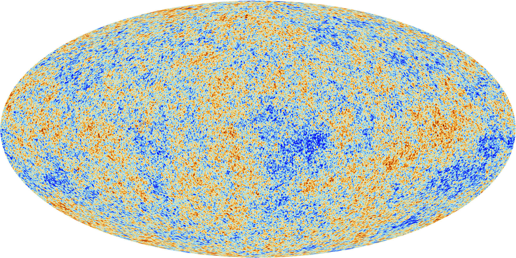
As we have discussed before, the plasma eventually cools sufficiently that the electrons bind with the protons and helium nuclei, so that the plasma transforms into a neutral gas. The universe becomes transparent and the thermal photons start freely streaming across the universe. Those photons that originated at just the right distance from us, and were headed our way, are arriving now. They give us an image of what the universe was like at the time of this transition in a thin spherical shell around us at a distance of about 46 billion light years that we call the last-scattering surface. Thus we have a means of studying the primordial plasma observationally. We saw maps of the CMB radiation in the previous chapter that revealed the monopole and the dipole. If we remove the monopole and the dipole then the remaining map is dominated by features that correspond to inhomogeneities on this last-scattering surface. A full-sky map of the CMB, as determined by data from the Planck satellite launched in 2009, is shown below. Planck flew later than WMAP but had higher angular resolution, increased sensitivity, and mapped the sky over a broader range of frequencies.

The following image is a projection of the spherical sky onto a 2D map. To better understand how this relates to what we observe from Earth, explore the virtual CMB planetarium below it by clicking and dragging. This shows how the CMB would look over a tree-lined horizon, if human eyes were extremely sensitive to light at millimeter wavelengths.

'

CMB Planetarium

The CMB Power Spectrum

So how do we learn things from a map of the CMB? Our theories do not actually predict the map. They predict statistical properties of the map. The most important statistical property is called the "power spectrum." The power spectrum tells us about the smoothness/roughness of the map, as a function of angular scale.

Qualitative Description

Now what does that mean, "as a function of angular scale?" Well, how would you describe the surface of the Pacific Ocean? Is it smooth or rough? The answer depends on length scale. On very large scales, scales much larger than the typical wavelength of a wave, it is quite smooth. But then on scales the length of a typical wave it is rougher. Zooming in further, to length scales smaller than a typical wave wavelength, it might appear smooth again.

Here, we'd also like to make very clear that we are not talking about the wavelengths of radiation emitted from the CMB. The power spectrum of the CMB refers to spatial wavelength of fluctuations in the temperature of the CMB across the sky.

We can do the same type of analysis with a map of the cosmic microwave background that we did with the Pacific Ocean. The scale-dependent measure of "roughness" we call "power." The power spectrum of the CMB is shown in the left panel below. The power is on the y-axis and the angular scale is shown on the x-axis. A higher multipole moment  \( \ell \) corresponds to a smaller scale. On the right panel is a simulated map that is consistent with this power spectrum. (Note that in all the following animations and pictures, each square shows an 8.5 x 8.5 degree patch of the CMB).

The y axis is power and the x axis is a measure of angular scale with larger scales on the left and smaller scales on the right.

Quantitative Description

Now let's give a more mathematical description of the power spectrum. Any function on the surface of a sphere, \(T(\theta, \phi)\) can be written as a sum over complex functions on the sphere with well-defined wavelengths, the spherical harmonics \(Y_{lm}(\theta,\phi)\):

\[T(\theta,\phi) = \sum_{lm} a_{lm} Y_{lm}(\theta,\phi).\]

The sum over \(l\) ranges from 0 to infinity and the sum over \(m\) ranges from \(-l\) to \(+l\). The \(l\) value tells you the wavelength of the oscillations: \(Y_{lm}(\theta,\phi)\) undergoes \(l\) oscillations as one runs through all 360 degrees of a great circle. The spherical harmonics for the lowest values of \(l\) have names: monopole, dipole, quadrupole and octupole are for \(l=0,1,2,3\) respectively. The figure below shows examples of dipole, quadrupole and octupole patterns over the whole sky (using the Mollweide projection for mapping the sphere on to a plane). Notice how larger multipoles like \( \ell = 3 \) correspond to smaller features on the CMB map, whereas lower multipoles like \( \ell = 1\) correspond to very large scale features.

Our cosmological models do not predict the temperature in a particular direction, or the value of a particular \(a_{lm}\); they predict statistical properties such as the mean and variance of \(a_{lm}\). For isotropic cosmologies, the mean of all except for the monopole is zero. The variance in isotropic theories is independent of \(m\) and given by

\[C_l \equiv \langle a_{lm}a^*_{lm} \rangle.\]

This variance, as a function of \(l\), is called the power spectrum. Rather than \(C_l\), we usually plot \(D_l \equiv l(l+1)C_l/(2\pi)\) instead. 

More Intuition of the Power Spectrum

Below, we show the same power spectrum and CMB map from above, but only features of the map whose scale falls within the grey box are included. At first, we see large scale features that increase in amplitude as the grey box passes over the first peak in the power spectrum at \(\ell\) of about 200. We then see progressively smaller features of lower amplitude as the box scans through the higher-\(\ell\) region. The pitch of the audio corresponds to the size of the features and the volume to the amplitude of the power spectrum in that range. We can hear the pitch increasing as we move from left to right. The volume rises as we pass over the first peak, then tapers off.

In the video below, the grey box steadily includes more of the power spectrum over time. As the box expands, we can hear more frequencies and see more features on the map.

 

Play "Match the Power Spectrum to the CMB"

First, observe each simulated CMB map. Next, click and drag to match the letter of the CMB map to the correct power spectrum on the left. Remember, large features correspond to power on the left of the power spectrum and small features correspond to power on the right side of the power spectrum. Feel free to refer back to the above videos. Warning: this is challenging. You will have to put some thought into it, and even then are likely to get it wrong the first time. If you do, think again and try again. I incorrectly assigned two of the power spectra the first time I tried it!

Matching Game

 

Comparison with Observations

Observations of the microwave background intensity as a function of direction on the sky have been carried out since the late sixties from telescopes on the ground, on high-altitude balloons, and from three different spacecraft (COBE, WMAP, and Planck). It is useful to get above the atmosphere as the atmosphere itself emits and absorbs at millimeter to submillimeter wavelengths, so balloons and spacecraft offer advantages. Ground-based instruments have been competitive though, in particular at higher angular resolution (higher \(\ell\)), which requires larger telescopes that are harder to lift above the atmosphere. One of the best ground-based sites for observing at millimeter to submillimeter wavelengths is at the South Pole, where the 10-meter South Pole Telescope (SPT) has operated since 2007. 

The WMAP satellite, like Planck, observed the full sky, whereas the SPT survey covered 2,500 square degrees, about 6% of the sky, but with lower noise and higher angular resolution. The figure below is from Story et al. (2013), showing the determination of the CMB temperature power spectrum from 7 years of WMAP observations and from the complete SPT 2500 sq. degree survey. The solid line is a fit to these spectra that includes the contribution from the CMB itself assuming the best-fit standard cosmological model (dashed line), and the contribution from other extragalactic sources of radiation.

The figure below is from the Planck Collaboration showing their determination of the CMB power spectrum and the predicted power spectrum of the standard cosmological model with its parameters adjusted to best agree with the data.  The lower panel shows the 'residuals': the data points after the best-fit model has been subtracted from it. It allows one to better inspect the quality of the agreement between theory and data. The small amplitude (relative to the error bars) of the departures from zero in the lower panel indicate agreement between theory and observation. Note that the y axis for the residuals is different for \(\ell < 30\) than it is for \(\ell > 30\). 

The agreement between observation and theory here is quite extraordinary. It gives us a very high level of confidence that we have a good understanding of the physical conditions of the universe when the scale factor was over 1,000 times smaller than it is today, around 14 billion years ago.

The Progression of CMB Power Spectrum Experiments

The following video tracks the progress of CMB measurements from 1967 to 2020. Gray boxes show the weighted average of prior measurements. The error bars indicate the type and quality of a measurement. The horizontal bar indicates the range of multipoles \( \ell \) over which the power measurement was taken. The vertical bar indicates the \( 1 \sigma \) error. (That means there is a 68% probability the true power lies within the vertical bar). If the error bar has a downward pointing arrow, it indicates that the experiment only determined an upper bound on the CMB power, not a detection.

Video Quiz