
Introduction
- Page ID
- 16398

Cosmologists speak with a high degree of confidence about conditions that existed billions of years ago when the universe was quite different from how we find it today: \(10^9\) times hotter than today, over \(10^{30}\) times denser, and much much smoother, with variations in density from one place to another only as large as one part in 100,000. We claim to know the composition of the universe at this early time, dominated almost entirely by thermal distributions of photons and subatomic particles called neutrinos. We know in detail many aspects of the evolutionary process that connects this early universe to the current one. Our models of this evolution have been highly predictive and enormously successful.
Einstein's Theory
It would be difficult to overstate the impact that Einstein’s 1915 General Theory of Relativity has had on the field of cosmology. So we begin our review with some discussion of the General Theory, and its origin in conflicts between Newtonian physics and Maxwell’s theory of electric and magnetic fields. We end our discussion of Einstein’s theory with its prediction that the universe must be either expanding or contracting.
Newton’s laws of motion and gravitation have amazing explanatory powers. Relatively simple laws describe, almost perfectly, the motions of the planets and the moon, as well as bodies here on Earth -- at least at speeds much lower than the speed of light. We use here the discovery of the planet Neptune as an example of their predictive power. Urbain Le Verrier, using Newton’s theory, was only able to explain the observed motion of Uranus if he posited the existence of a planet with a particular orbit, an extra planet beyond those known at the time. Following up on his prediction, Johannes Gottfried Galle and John Couch Adams looked for a new planet where Le Verrier said it was to be found and, indeed, there it was.
Less than 20 years after the discovery of Neptune, a triumph of the Newtonian theory, came another great inductive synthesis: Maxwell’s theory of electric and magnetic fields. The experiments that led to this synthesis, and the synthesis itself, have enabled the development of a great range of technologies we now take for granted such as electric motors, radio, television, and cell phones. More important for our subject, they also led to radical changes to our conception of space and time.
These radical changes arose from conflicts between the synthesis of Maxwell with that of Newton. For example, in the Newtonian theory velocities add: if A is sees B move at speed v to the west, and B sees C moving at speed v to the west relative to B, then A sees C moving at speed v+v = 2v to the west. But one solution to the Maxwell equations is a propagating disturbance in the electromagnetic fields that travels with a fixed speed of about 300,000 km/sec. Without modification, the Maxwell equations seem to predict that both A and B would see electromagnetic wave C moving away from them at a speed of 300,000 km/sec, violating the velocity addition rule that one can derive from Newtonian concepts of space and time.
Einstein’s solution to these inconsistencies includes an abandonment of Newtonian concepts of space and time. This abandonment, and discovery of the replacement principals consistent with the Maxwell theory, happened over a considerable amount of time. A solution valid in the absence of gravitation came out first in 1905, with Einstein’s paper with (translated) title “On the Electrodynamics of Moving Bodies.” His effort to reconcile gravitational theory with Maxwell’s theory did not fully come together until November of 1915, with a series of lectures in Berlin in which he presented his General Theory of Relativity.

One indicator that Einstein was on the right track was his realization, in September (check) 1915, that his theory provided an explanation for a longstanding problem in solar system dynamics known as the anomalous perihelion precession of Mercury. Given Newtonian theory, and an absence of other planets, Mercury would orbit the Sun in an ellipse shape. However, the influence of the other planets is to make Mercury follow almost an ellipse, in a pattern that is well approximated as that of a slowly rotating ellipse. One way of expressing this rotation is to say how rapidly the location of closest approach, called perihelion, is rotating around the Sun. Mercury’s perihelion precession is quite slow. In fact, it’s less than one degree per century. More precisely, it’s 575 seconds of arc per century, where a second of arc is a degree divided by 3,600 (just as a second is an hour divided by 3,600).
Urbain Le Verrier, following his success with Neptune, took up the question of this motion of Mercury: could the perihelion precession be understood as resulting from the pulls on Mercury from the other planets. He found that he could ascribe about 532 seconds of arc to the other planets, but not all of it. There is an additional, unexplained (“anomalous”) precession of 43 seconds of arc per century. Le Verrier, of course, knew how to handle situations like this. He proposed that this motion is caused by a not-yet-discovered planet. This planet was proposed to have an orbit closer to the Sun than Mercury’s and eventually had the name Vulcan.

But “Vulcan, Mercury, Venus, Earth, Mars, Jupiter, Saturn, Uranus, Neptune, Pluto” is probably not the list of planets you learned in elementary school. Unlike the success with Neptune, Newtonian gravity was not going to be vindicated by discovery of another predicted planet. Rather than an unaccounted-for planet, the anomalous precession of Mercury, we now know, as Einstein figured out in September of 1915, is due to a failure of Newton’s theory of gravity. At slow speeds and for weak gravitational fields the Newtonian theory is an excellent approximation to Einstein’s theory -- so the largest errors in the Newtonian theory show up for the fastest-moving planet orbiting closest to the Sun.
Amazingly, thinking about a theory that explains experiments with electricity and magnets, and trying to reconcile it with Newton’s laws of gravitation and motion, had led to a solution to this decades-old problem in solar system dynamics. The theory has gone on from success to success since that time, most recently with the detection of gravitational waves first reported in 2016. It is of practical importance in the daily lives of many of us: GPS software written based on Newtonian theory rather than Einstein’s theory would be completely useless.
More important to our subject, Einstein’s theory allowed for more-informed speculation about the history of the universe as a whole. In the years following Einstein’s November 1915 series of lectures, a number of theoreticians calculated solutions of the Einstein equations for highly-idealized models of the universe. The Einstein field equations are extremely difficult to solve in generality. The first attempts at solving these equations for the universe as a whole thus involved a great deal of idealization. You might call it the “most spherical cow approximation of all time.” They approximated the whole universe as completely homogeneous; i.e., absolutely the same everywhere. 
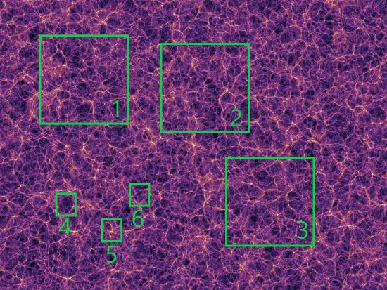
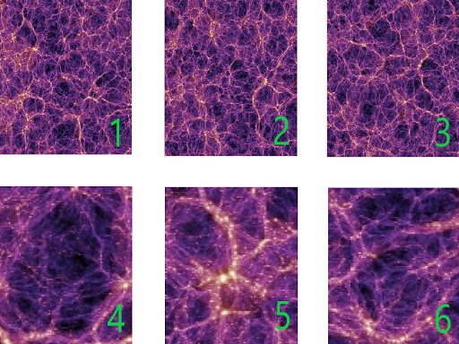
We now know that on very large scales, this is actually a good approximation to our actual universe. To illustrate what we mean by homogeneity being a good approximation on very large scales, we have the figure below which slows a slice from a large-volume simulation of the large-scale structure of our universe. The image has two sets of sub-boxes: large ones and small ones. We can see that the universe appears different in the small boxes. Box 4 is under dense, Box 5 is over dense, and Box 6 is about average. If we look at the larger boxes, the universe appears more homogeneous. Each box looks about the same. This is the sense by which we mean that on large scales the universe is highly homogeneous.
Prediction of Expansion (or Contraction) of space (above)
Gif of an expanding grid (below) Image by Alex Eisner
D vs. z: Low z
In 1929, Edwin Hubble made an important observation by measuring distances to various galaxies and their redshifts. Hubble inferred distances to galaxies by using standard candles, which are objects with predictable luminosities. Since farther away objects appear dimmer, one can predict distances by comparing the object’s expected luminosity with how bright it appears. The redshift of a galaxy, which cosmologists label as “z”, tells us how the wavelength of light has shifted during its propagation. Mathematically, 1+z is equal to the ratio of the wavelength of observed light to the wavelength of emitted light: \(1+z = \lambda_{observed}/\lambda_{emitted}\). At least for low z, one can think of this as telling us how fast the galaxy is moving away from us according to the Doppler Effect: a higher redshift indicates a larger velocity via \(v=cz\) where \(c\) is the speed of light. If a galaxy were instead moving towards us, its light would appear blueshifted. Hubble found that not only were nearly all the galaxies redshifted, but there was a linear relationship between their distances and redshifts. This is represented by Hubble’s law, v=\(H_0\)d. This simple law had large consequences for our understanding of the cosmos: it indicated that the universe was expanding.
To understand this, take a look at the image of an expanding grid. Each of the two red points is “stationary”; they each have a specific defined location on the grid and do not move from that location. However, as the grid itself expands, the distance between the two points grows, and they appear to move away from each other. If you lived in the center of this expanding grid, you would see all other points moving away from you. Try placing your mouse over different points on the grid and following them as they expand. You will notice that points farther from the center will move away faster than points close to the center. This is how Hubble’s law and the expansion of space works. Instead of viewing redshifts as being caused by a Doppler effect from galaxies moving through space, we will come to understand the redshift as the result of the ongoing creation of new space.
Hubble’s constant, \(H_0\), tells us how fast the universe is expanding. It was first estimated to be about 500 km/s/Mpc, but after eliminating some large systematic errors and obtaining more accurate measurements, we have narrowed it down to about 67 to 74 km/s/Mpc. This means that on large length scales, where the approximation of a homogeneous universe becomes more accurate, about 70 kilometers of new space are created per second in every Megaparsec.
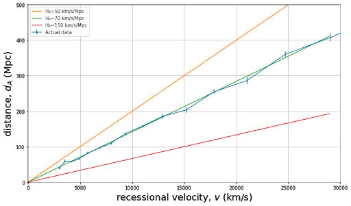
Figure A: Hubble’s law shown for low redshifts, where we can think of the redshift as arising due to a Doppler effect and so v=cz. The blue data points are distances inferred from observations of supernovae and the green line is a best-fit line for a Hubble constant of 70 km/s/Mpc. Orange and red lines show how this relationship would differ for other Hubble constants. Image by Adrianna Schroeder.
D vs. z: High z
As we will see, from Einstein’s theory of space and time we can expect the rate of expansion of space to change over time. The history of these changes to the expansion rate leaves their impact on the distance-redshift relation if we trace it out to sufficiently large distances and redshifts. As we measure out to larger distances, the relationship is no longer governed by cz = \(H_0\) d. Instead, we will show that the redshift tells us how much the universe has expanded since light left the object we are observing.
\[1+z = \dfrac{ \lambda_{observed}}{ \lambda_{emitted}} = \dfrac{ a_0}{a_e}\]
where a is the “scale factor” that parameterizes the expansion of space, \(a_0\) is the scale factor today and \(a_e\) is the scale factor when the light was emitted. We can observe quasars so far away that the universe has expanded by a factor of 7 since the light left them that we are receiving now. For such a quasar we have \(a_0\)/\(a_e\) = 7 so the wavelength of light has been stretched by a factor of 7, and by definition of redshift \(z\) we have \(z = 6\).
The distance from us to such a quasar depends on how long it took for the universe to expand by a factor of 7. If the expansion rate were slower over this time, then it would have taken longer, so the quasar must be further away. Measurements of distance vs. redshift are thus sensitive to the history of the expansion rate.
As we will see, how the expansion rate changes over time depends on what the universe is made out of. Therefore, studying \(D\) vs. \(z\) out to high distances and redshifts can help us determine the composition of the universe. We can see such measurements in Fig. B, together with some model curves. The models all have the same expansion rate today, \(H_0\), but differ in the mix of different kinds of matter/energy in the universe. A model that’s purely non-relativistic matter, the green dashed line, does a very poor job of fitting the data. The data seem to require a contribution to the energy density that we call “vacuum energy” or “the cosmological constant.” The “Lambda CDM” model has a mixture of this cosmological constant and non-relativistic matter. The cosmological constant causes the expansion rate to accelerate. Thus, compared to the model without a cosmological constant, the expansion rate in the past was slower, it thus took a longer time for the universe to expand by a factor of 1+z, and thus objects with a given z are at further distances. This acceleration of the expansion rate, discovered via \(D\) vs. \(z\) measurements at the end of the 20th century, was a great surprise to most cosmologists. Why there is a cosmological constant, or whether there is something else causing the acceleration, is one of the great mysteries of modern cosmology.
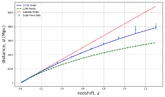
Figure B: Redshift versus distance up to higher redshifts. The shape of the graph can tell us about the contents of the universe--current data best fits the “Lambda-CDM” model, which we will learn about later. Note: we use z here for our x axis rather than the recessional velocity \(v = cz\). Although for low \(z\), we can think of redshift as arising from a Doppler effect, that interpretation only makes sense for \(z << 1\). More generally, as we will see, \(1+z\) is the amount by which the universe expands since light left the object we are observing. Image by Adrianna Schroeder.
He/H vs. O/H
The expansion of the universe implies that it must have been much smaller, and much denser, in the past. If this is true, we should be able to see some consequences from the very high density period of the early universe. One such consequence is the abundances of light elements we see today, or the ratios of helium to hydrogen, and oxygen to hydrogen.
We usually think of heavy elements as a product of nucleosynthesis (formation of nuclei) in stellar fusion and supernovae. Over billions of years of stellar processing and an overall increase in heavy element abundances, the chemical abundances of stars become richer with elements besides hydrogen, such as helium, oxygen, and iron. In a given star, we typically see a direct correlation between its oxygen abundance and iron abundance. If a star is oxygen-rich, it is likely a newer star made from dust clouds containing heavier elements, and thus likely has a high iron content as well. We can see this relationship in Figure C, which plots the oxygen and iron content of many stars. This observed relationship supports our hypothesis that these elements were formed together over time with stellar processing.
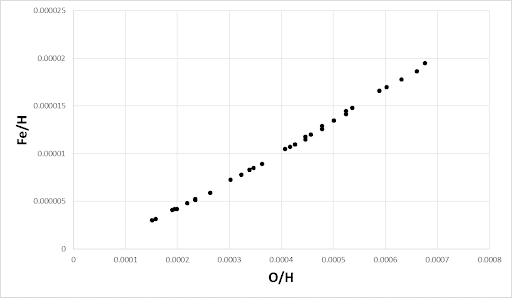
Figure C: Relative abundances of oxygen-to-hydrogen and iron-to-hydrogen. We see a trend in which low-iron stars tend to have low-oxygen, while iron-rich stars are also oxygen-rich. This is because iron and oxygen were formed together over billions of years of stellar processing.
Observations of helium abundances gives us a different relationship, which can be seen in Figure D. As with iron and oxygen, an oxygen-rich star is likely to contain more helium, which indicates that both helium and oxygen have been created over time with stellar processing. The difference is that we see a significant abundance of helium even in very old stars formed by gas clouds containing little to no heavy elements. This points to a primordial abundance of helium that existed even before stellar processing. Where did this helium come from?
In 1948, Gamow explored the very early universe as a source of elements heavier than hydrogen. He extrapolated Einstein’s theory of an expanding universe with certain assumptions of what the universe is made of, and concluded that the universe was infinitely dense at a finite time in the past. He theorized that this early universe could be a prodigious source of heavier elements. If the universe began at infinitely high density and temperatures and underwent rapid expansion and cooling, atomic nuclei would form within a window of just a few minutes. Before this window, high-energy radiation did not permit any nuclei to survive, and after this window, temperatures were too low for the nuclear collisions to overcome the Coulomb repulsion.
In order to avoid overproduction of helium and heavier elements, Gamow and his collaborator Alpher concluded that the ratio of nucleons to photons had to be small. Since the number of photons in black body radiation is proportional to temperature cubed, this means that the “Big Bang” had to be very hot. From these considerations, Alpher and Herman theorized that we should see a background of heat and light from this period of high temperature and photon density. This background was discovered later in 1964 and is known as the Cosmic Microwave Background.
Figure D: Relative abundances of oxygen-to-hydrogen and helium-to-hydrogen in stars. While there is still a trend in which stars with low O/H also have lower He/H, even the most oxygen-poor stars contain a significant abundance of helium. This is because all these objects formed with a primordial abundance of helium, whereas there is essentially no primordial abundance of oxygen. (Ned Wright, UCLA)
Map of the CMB
- Mostly a visual section with some explanation
- CMB shows universe when it was very young, and very simple. (High degree of uniformity/ homogeneity - 1 part in 100,000)
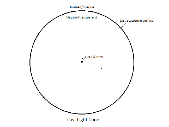
- Diagram of past light cone- show where/when the CMB came from
- Photons could not travel freely until the universe had expanded and cooled such that protons and neutrons combined to make atoms. These photons have traveled since this last-scattering and redshifted with the expansion of the universe. The ones that reach us now are 46 billion light years away in the microwave spectrum of light (temp = 2.7K)
 Although its existence had been predicted around 1950, the Cosmic Microwave Background was discovered in 1964. It was uncovered by accident while two radio astronomers, Arno Penzias and Robert Woodrow Wilson, were experimenting with an ultra-sensitive radio antenna. Even after removing all known possible sources of noise and interference, they detected a consistent noise of microwave radiation coming from all directions, day and night. They inferred that this noise had to be coming from a source outside our galaxy. The characteristics of this radiation perfectly fit predictions for the Cosmic Microwave Background, a background of radiation left over from the Big Bang that permeates all of space.
For the first few hundred thousand years, the universe was opaque because photons were constantly scattered off free electrons, unable to travel freely. As the temperature decreased, matter was able to recombine into atoms, and electrons bound to nuclei. Photons stopped scattering and were now able to travel freely: this time period is called the Recombination Era. Those same photons have traveled across the universe ever since this time, and the CMB we observe is the photons that are just now reaching us. The region of space where they started traveling freely, we call the “surface of last scattering,” a receding spherical shape around the observer which is the boundary on our past light cone between when the universe was opaque and when the universe became transparent.
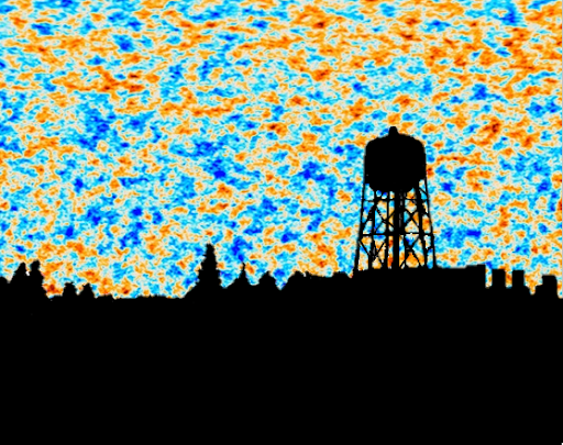
The CMB currently has a temperature of about 2.73 K, cooled by the expansion of space by over a factor of 1000 since the time it was released, and is uniform to 1 part in 100,000. If one had eyes highly sensitive to microwave radiation, the above image shows how the sky over Chicago would look, with the colors encoding tiny variations in brightness. The high degree of uniformity reflects the high degree of uniformity in the early universe. The small departures from uniformity eventually grew over time to produce the diversity of structures we see in the universe today. Without these departures from uniformity there would be today no galaxies, stars, planets, or physics students.
As we have seen above, the CMB was predicted based on consideration of production of light elements when the universe was just a few minutes old, very hot, and expanding very rapidly. It is thus strong evidence in support of a hot, dense, and rapidly expanding phase of the evolution of the universe; i.e., a Big Bang.
Cosmic Pie Chart
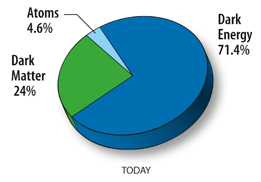 We know this now from data like the above and our knowledge of physics
- We obtain a lot of information from light freely falling down on us, and we can interpret this information by using simple natural laws that we know to be true from laboratory experiments here on Earth
- The standard cosmological model has this particular mix of ingredients
Conclusion / Wrapping It Up
- The agreement between cosmological predictions and observations give us a high degree of confidence. However, we still don’t know what most of the universe is made of, and there are many more mysteries remaining to be solved.
- Examples: dark matter, cause of cosmic acceleration, how did Big Bang begin
- Our measurements are constantly improving, and one never knows when a combination of precise measurements and predictions will reveal something new and interesting about the universe
Assignment: Write a brief summary of the contents of the chapter.