4.2: Work and Pressure

Last updated
Save as PDF

Page ID: 19177

\( \newcommand{\vecs}[1]{\overset { \scriptstyle \rightharpoonup} {\mathbf{#1}} } \) \( \newcommand{\vecd}[1]{\overset{-\!-\!\rightharpoonup}{\vphantom{a}\smash {#1}}} \)\(\newcommand{\id}{\mathrm{id}}\) \( \newcommand{\Span}{\mathrm{span}}\) \( \newcommand{\kernel}{\mathrm{null}\,}\) \( \newcommand{\range}{\mathrm{range}\,}\) \( \newcommand{\RealPart}{\mathrm{Re}}\) \( \newcommand{\ImaginaryPart}{\mathrm{Im}}\) \( \newcommand{\Argument}{\mathrm{Arg}}\) \( \newcommand{\norm}[1]{\| #1 \|}\) \( \newcommand{\inner}[2]{\langle #1, #2 \rangle}\) \( \newcommand{\Span}{\mathrm{span}}\) \(\newcommand{\id}{\mathrm{id}}\) \( \newcommand{\Span}{\mathrm{span}}\) \( \newcommand{\kernel}{\mathrm{null}\,}\) \( \newcommand{\range}{\mathrm{range}\,}\) \( \newcommand{\RealPart}{\mathrm{Re}}\) \( \newcommand{\ImaginaryPart}{\mathrm{Im}}\) \( \newcommand{\Argument}{\mathrm{Arg}}\) \( \newcommand{\norm}[1]{\| #1 \|}\) \( \newcommand{\inner}[2]{\langle #1, #2 \rangle}\) \( \newcommand{\Span}{\mathrm{span}}\)\(\newcommand{\AA}{\unicode[.8,0]{x212B}}\)

Work revisited

We introduced work in Chapter 2 for a total force acting on an object over some displacement of the object:

\[ W = \int \limits_A^B \overrightarrow F_{net} \cdot \overrightarrow {ds}\label{workDef.int}\]

There are several special cases that are worth noting. First, when the force is constant and is parallel to the displacement \(x\), the above equation simplifies to:

\[ W = Fx\]

The next simplest case is when the force is a linear function of \(x\). For example, \( F(x) = kx \) for a spring. In this case, work then becomes:

\[ W = k \int\limits_{x_i}^{x_f} x dx = \dfrac{1}{2} k (x_{f}^{2} - x_{i}^{2})\label{work.spring}\]

Graphical Interpretation of Work

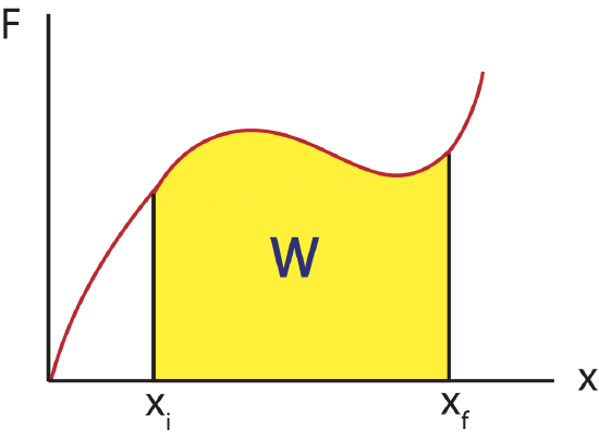
If a force \(F(x)\) is plotted as a function of \(x\), there is a very simple interpretation of the definite integral in the above equation: the work, \(W\), is simply the area under the \(F(x)\) curve. This should come as no surprise to anyone who has studied integrals. The figure below illustrates a force that varies with position (red curve), and the area in the yellow region is the work done over the interval \(x_i\) to \(x_f\).

Figure 4.3.1: Work for a variable force.

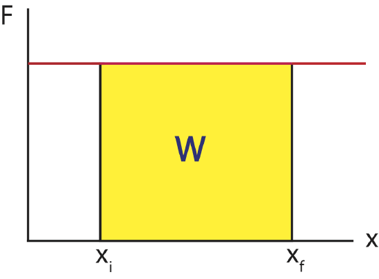
Examining the aforementioned special cases in this graphical way reveal the simplicity and utility of the graphical approach. The graph of a constant force is a horizontal line as shown below. The region under a line is a rectangle, whose area is simply \(W=F \Delta x=F(x_f-x_i) \).

Figure 4.3.2: Work for a constant force.

A linear force describes the behavior of simple springs and sometimes pendulums, and is the basis for the simple harmonic oscillator, a widely applicable model. To find the work done graphically, we must compute the area of the yellow region below, which in this case is a trapezoid. There is an area formula for a trapezoid, which is \( A = \dfrac{h_1 + h_2}{2} b \), where the base \(b=x_f-x_i\). Or you can treat this area as a sum of the areas of a rectangle \( A_1 = h_1 b\) and a triangle \( A_2 = \dfrac{1}{2}(h_2-h_1) b\). Adding the two areas results in the exact equation for an area of a trapezoid.

Figure 4.3.3: Work for a linear force.

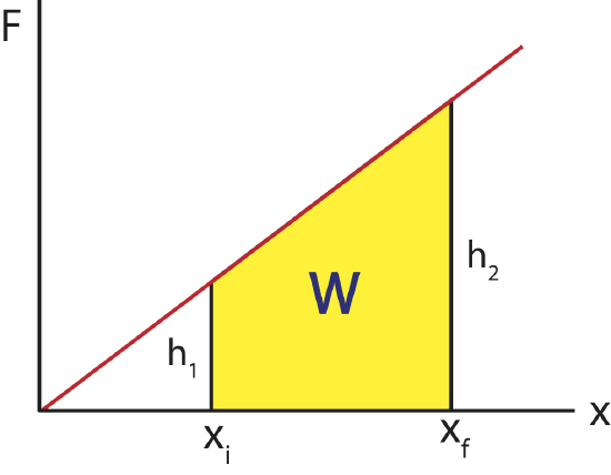
Calculating work directly from the graph, remember that the functional form of force is \( F(x)= kx \), thus \(h_1\) is \( F(x_i)= kx_i \), and \(h_2\) is \( F(x_f)= kx_f \). Then we have:

\[ W = \dfrac{h_1 + h_2}{2} b=\dfrac{kx_i + kx_f}{2} (x_f-x_i)=\dfrac{k}{2}(x_f+x_i) (x_f-x_i)=\dfrac{k}{2}(x^2_f-x^2_i)\]

This is identical to Equation \ref{work.spring} for work done by a linear force that we obtain above by performing direct integration.

Rather than the integral expression for work, it is often convenient to use a differential expression. That is, we want to talk about the small increment of work corresponding to the product of the parallel component of force and the differential increment of distance, \(dx\).

Figure 4.3.4: Work for a differential increment of distance

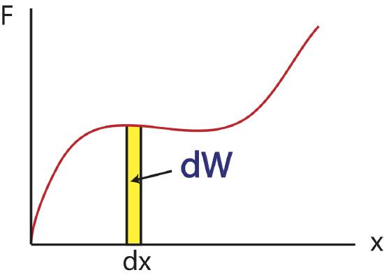
This expression for the incremental work, \(dW=F(x)dx\), fits nicely with the graphical representation of work and the graphical interpretation of the definite integral. If you do not remember this from your calculus class, you might want to go back and review it over the next couple of weeks. (The graphical interpretations of derivatives and integrals are two of the those important concepts that you should take away from calculus, i.e., things you remember for the rest of your life.)

Work Done on a Fluid

We now have a general expressions for work in terms of forces and distances moved. But when you push on a fluid (i.e., a liquid or a gas), it is more useful to describe this force in terms of pressure. The force exerted on a fluid by an object of cross-sectional area A is proportional to the pressure P and area A and is directed in a direction perpendicular to A. This is illustrated in the figure below.

Figure 4.3.5: Animation of pressure on a fluid.

The force pushing the movable piston to the right is equal to the force the fluid contained in the cylinder exerts on the piston to the left. The magnitude of this force is not a definition of pressure, but simply the relation of force to pressure:

\[ P = \dfrac{F}{A} \]

The dimensionality of pressure is force per area, which is also energy per volume:

\[ \text{Pressure} = \dfrac{\text{Force}}{ \text{length}^2} = \dfrac{\text{Energy}}{ \text{length}^3} = \dfrac{\text{Energy}}{\text{volume}}\nonumber\]

The units of pressure in SI are the Pascal (Pa):

\[\text{Pressure} = \dfrac{N}{m^2}=\dfrac{J}{m^3}=\text{Pascal}\nonumber\]

Some useful conversions involving pressure are:

\[1.0 atm = 1.01 \times 10^{5} Pa = 14.7 \dfrac{lb}{in^{2}} (psi) \nonumber\]

Our previous expressions for work were in terms of the linear distance, a product of force and displacement. However, when dealing with fluids, it is useful to make a change of variables from \(x\) to \(V\). For the case of a piston, the relation between the differentials \(dV\) and \(dx\) is illustrated in the figure below.

Figure 4.3.5: Animation of work done on a fluid

Note: The reason for the minus sign in front of dV is because the volume gets smaller as “x” increases.

To extend the definition of work to fluids using \(V\) and \(dV\) rather than \(x\) and \(dx\), use \( dV = -Adx \) to make the change of variables. Substitute \(\dfrac{-dV}{A}\) for \(dx\) and use the relationship between force, pressure, and area to substitute \(F(x) \) for \(P(V) A \), and the integral becomes:

\[ W = - \int\limits_{V_i}^{V_f} P(V) dV \]

This is the expression for the work done on a fluid when it is compressed from a volume V_i to a volume V_f. The minus sign in front of the integral ensures that when the fluid is being compressed (\(dV\) is negative), work comes out positive, since work is being done on the system. If instead of being compressed, the volume expands, the work done on the fluid will be negative since \(dV\) is positive, since the fluid does positive work on some other physical system or work is being done by the system.

In a special case is when work being done is at constant pressure, work simplifies to:

\[W = -P\Delta V \]

Since the area under a F(x) vs. x plot gave us work done, the area under a P(V) vs. V plot will give us the work done on or by the gas. We will explore this idea in greater detail in Section 4.4.

Contributors

Authors of Phys7A (UC Davis Physics Department)