2.7: Force and Potential Energy

Spring-Mass Force

There is a deep connection between force and potential energy. This relationship has a useful graphical representation that will help us better understand the spring-mass potential energy and, in Chapter 3, the potential energy associated with the bonding between atoms.

Graphed below is the potential energy of a spring-mass system vs. deformation amount of the spring. As was explained earlier, this is a second degree, or parabolic relationship. Marked on the figure are the positions where the force exerted by the spring has the greatest and the least values.

Figure 2.7.1: spring-mass forces at different displacements from equilibrium

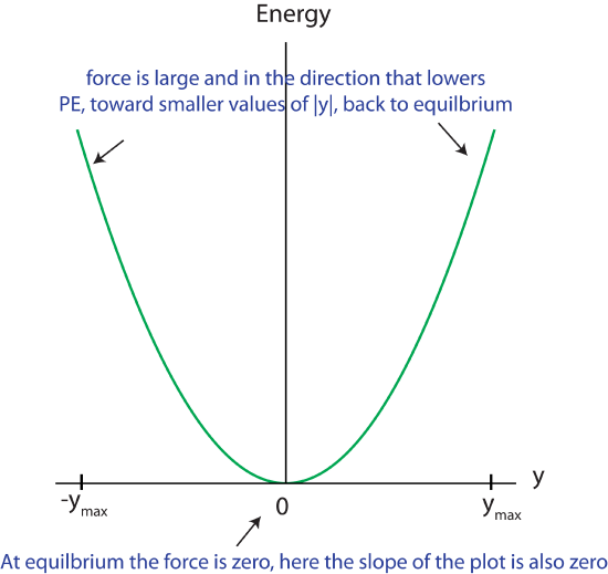
If pulled or pushed to some value of the position y, we know intuitively that the spring will try to snap back to its original shape -- that is, that it will tend to return to zero deformation. We also know that it takes more force to deform the spring as you go further from equilibrium. How can we confirm our intuitions from the graph? Mathematically, we have already described this type of force using Hooke's Law: \(F=-kx\). Now let us go backward and see what we can learn about force directly from potential energy.

Force and Potential Energy Connection

We see from our understanding of behavior of the spring and from Figure 2.7.1 that the force is largest away from equilibrium, which is where the slope of the PE_sm plot is the largest as well. The force also points toward decreasing potential energy, or toward smaller values of |y|. At equilibrium the slope of the plot is zero, which is where there is also no force acting on the spring-mass. This clear connection we are seeing between the slope of PE_sm vs. y plot and magnitude of force, and the direction of force pointing toward decreasing PE_sm, turns out to be universal. Mathematically these relationships are written as:

\[ F_{x} = -\frac{dPE}{dx} \label{force.PE}\]

The subscript "x" refers to the component of the force vector pointing in the "x" direction. For a one-dimensional force, such as the force of gravity which always points down toward the -y direction, or the spring-mass force which always points in the -|x| direction, you may drop the subscript. This is a general result that is true for the force associated with any potential energy.

The derivative of a function f(x), \(\frac{df}{dx}\), at some values of x represents the slope of the f(x) vs x plot at the particular values of x. Thus, graphically Equation \ref{force.PE} means that if we have potential energy vs. position plot, the force is the negative of the slope of the function at some point:

\[ F = -(slope) \]

Disregarding the minus sign for a moment, this tells us that the steeper the slope of a PE curve plotted against its position variable, the greater the magnitude of the force. The restoring force of the spring (or anything that oscillates) will be zero when the slope is zero, which occurs at the equilibrium point, i.e., where the object comes to rest when it stops vibrating.

The minus sign means that if the slope is positive, the force is toward the negative direction (-x), and visa versa. This should make sense, because it says that the force will try to push the object back to lower potential. If it were the other way around, springs would stretch themselves out spontaneously and planets would fly away from each other! For example, looking back at Figure 2.7.1, we see that the slope of the plot on the positive side of y (spring is stretched) is positive, which will give us a negative force. Recalling that force is a vector, so the negative sign for a one-dimensional force tells us that it points toward the negative direction. If the spring is stretched (y>0), this result tell us that the force point in the (-y) direction, thus toward lower values of y (and lower values of PE_sm) back to equilibrium. On the other side of the plot when the spring is compressed, slope is negative, giving us a force pointing toward +y direction, which is where the equilibrium is and toward lower values of PE_sm. This is consistent with behavior of the spring which pulls back when stretched and pushes back when compressed.

To summarize, we learned two very important points here:

• magnitude of force is equal to the magnitude of the slope of potential energy as a function of position graph.
• force points in the direction of decreasing potential energy.

We can quantitatively show just how correct this relationships is. If we take our spring-mass potential energy function, then the force is:

\[F_{y} = -\frac{PE}{dy} = -\frac{d}{dy} (\frac{1}{2}ky^{2}) = -ky \]

The final result is Hooke's Law, the first equation introduced in our discussion of springs! Now that you're convinced that this relationship is real, let's see if we can understand why.

Using What We Know

It all boils down to the concepts of work and energy conservation, we have been using in the Energy-Interaction Model. To see this, consider the following situation (pictured below). Imagine a box is lifted through a force field (we use a general word "field" here to refer to a force that can be defined everywhere in space), like lifting an object against gravity. Imagine also that the force is constant and pointing downwards at all points in space.

Figure 2.7.2: forces that result in a change of potential energy.

As described in the figure above, the box is being lifted at a constant kinetic energy. The work cannot be going to kinetic energy, but it is being transferred to potential energy. The amount of work I do on the object is given by the force I exert times the distance I moved it:

\[W = F_{me} \Delta y \]

The "object" exerting \(F_{field}\) is part of the physical system, since it is interacting with the object that was moved resulting in a change of potential energy. Thus, the force only I exert (outside "object") contributes to the amount of potential energy the object gains. We can therefore replace the amount of work done by me with the amount of potential gained, \(W=\Delta PE \). Solving for \(F_{me}\), we get:

\[F_{me} = \frac{ \Delta PE}{ \Delta y} \]

However, what we wish to know is not the force I exerted, but the force the field exerted, since it is exactly that force between two objects (box and Earth in this example) that defines the potential energy between them. Since the box is moving at constant speed the forces must be balanced. Thus, the force the field exerts is equal and opposite the force I exert:

\[F_{field} = - \frac{ \Delta PE}{ \Delta y} \]

To derive this result, we used constant force field (gravity near the surface of the Earth). But this applies even to changing forces. As \(\Delta\)'s become sufficiently small \(\frac{ \Delta PE}{ \Delta y}\) becomes a derivative, \(\frac{dPE}{dy}\), which is precisely the slope of potential energy as a function of y.

Everything we say here about the relation of force to potential energy is strictly true when the force depends on only one spatial dimension. That is, we consider the spring to move in only one direction in space or gravity only pointing down. It the force depends on movement in two or three dimensions, then technically the force is the negative of the gradient of the potential:

\[ \overrightarrow F = -\overrightarrow \nabla PE \]

The gradient operator \(\nabla\) is short-hand for writing:

\[ F_{x} = -\frac{dPE}{dx};~~F_{y} = -\frac{dPE}{dy};~~F_{z} = -\frac{dPE}{dz}\]

where x, y, and z are variables for the three spatial dimensions. This is analogous to releasing a ball on a smooth hillside; the ball starts to roll in the direction of the steepest slope of the hill. In two or three dimensions, the force is the derivative of the potential in the direction of “steepest slope".