5.4: Electric Circuits

From Fluid to Electric Charge Flow

Another type of steady-state system is the flow of electric charge in an electric circuit.  Although, they are seemingly very different system as we will shortly see, the application of energy conservation to electric flow results in an analogous model to that of fluid flow. Instead of a fluid flowing, current electricity (as opposed to static electricity) involves the flow of electric charge. To create intensive energy systems we divide energy by electric charge, rather than by volume as we did for fluids.

Fluid Circuits

The examples we worked through in Section 5.3 have shown how we can use the steady-state energy-density model to calculate various fluid flow parameters given sufficient details about the physical situation. We have mostly focused on segments of a fluid system where there are changes in the physical properties of the system that result in changes in energy-density or addition of energy with a pump or dissipation of energy due to resistance. Now we extend this analysis to circuits. We begin by summarizing the components of the steady-state energy-density model we developed in the context of fluids and which we will now generalize to the flow of electric charge. The complete energy-density Equation 5.3.11 as applied to fluid phenomena is given by:

\[\Delta (\text{total head}) = \frac{E_{pump}}{V} – I R\label{fluid-head}\]

The above equation states that the change in the total fluid energy-density as we move from one point to another point in the stead-state flow will increase due to energy added by a pump and will decrease due to the transfer of fluid energy-density to thermal energy-density.

Let us define a fluid circuit to represent a system where the fluid flows in a circular manner or in a loop as shown in Figure 5.4.1 below. 

Figure 5.4.1: Fluid Circuit.

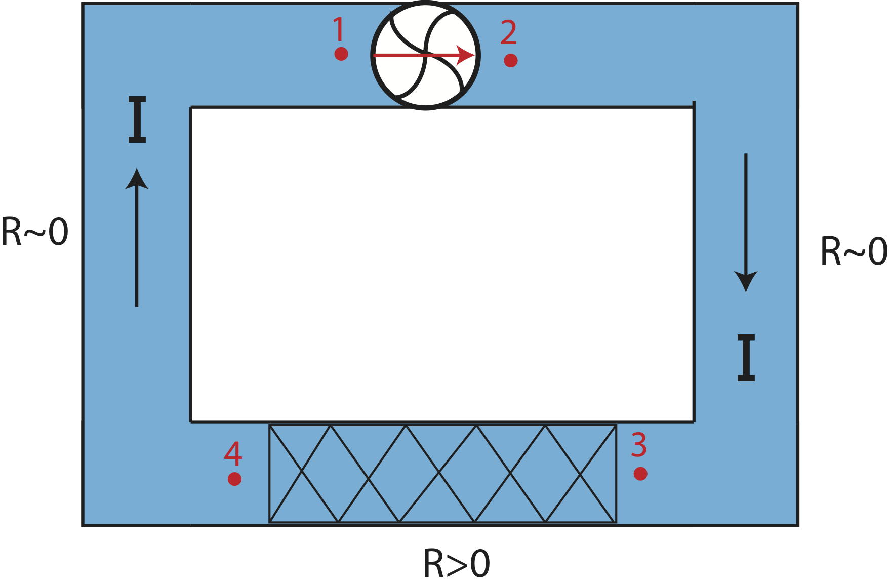
The fluid circuit above has a pump between points marked 1 and 2.  The pump pushes the fluid to the right causing a current, \(I\), in the clockwise direction.  We will assume that only one section of the pipe system between points marked 3 and 4 has significant resistance, \(R>0\), and the pipe in the rest of the circuit has negligible resistance, \(R\sim 0\). (We do this to make a clear analogy to electric circuits as you will see below.)  The view of the circuit above is a top view so that the pipe is horizontal throughout the entire circuit. Thus, there is no change in gravitational potential energy-density anywhere along the circuit. The pipe also has uniform area throughout, so the Equation \ref{fluid-head} for this circuit simplifies to:

\[\Delta P= \frac{E_{pump}}{V} – I R\]

The pressure difference in the equation above depends on which particular part of the circuit being analyzed. Let us analyze the energy-density changes for the specific locations, 1-4, shown in the circuit in Figure 5.4.1.

Across the pump:

\[P_2-P_1=\frac{E_{pump}}{V}\]

Across the pipe with negligible resistance:

\[P_3-P_2=0;~~~~P_1-P_4=0\]

Across the pipe with non-zero resistance:

\[P_4-P_3=-IR\]

If we were to add the four equations above that would analyze the entire circuit going from 1 and back to 1 clockwise in the direction of the current. Adding up the left-hand-sides of the four equations, we find they add up to zero.  This is because we went around the entire circuit and returned back to the original location "1".  Since energy-density is conserved in a steady-state system, the pressure at location 1 is fixed, energy cannot be created or destroyed. In other words, \(\Delta P=0\) when going around the circuit.  Adding the right-hand side of the 4 equations above we arrive at:

\[0=\frac{E_{pump}}{V}-IR\]

Rearranging we find that:

\[I=\frac{E_{pump}/V}{R}\label{current-pump-R}\]

As was stressed in Section 5.3 although the current in a steady-state system is the same everywhere within that system, the value of that constant current depends on the strength of the pump and the amount of resistance present. Equation \ref{current-pump-R} demonstrates exactly that. The larger the strength of the pump the larger the current, while the more resistance the system has the smaller the overall current. In Section 5.3, we have treated the current as an independent variable, as we looked at drops in total head for fluid systems. However, frequently, we deal with complete circuits. The current is no longer an independent variable, but rather the resistance(s) and pump(s) determine the current that exists in the circuit.

Electric Circuits

The electric circuit depicted in Figure 5.4.2 below is analogous to the fluid circuit in Figure 5.4.1. Instead of fluid flowing through pipes, electric charge is flowing through wires. Wires are depicted as a straight lines making right angles as charges move through them in a circuit. The "mechanism" that adds energy to the system is a battery or a power source labeled as \(\mathcal{E}\) in the circuit below, which  stands for emf or electromotive force of that power source. The analogous mechanism in the fluid circuit is the pump which adds energy to the system and allows the fluid to flow. In a fluid circuit where the pipes are horizontal, the fluid would not flow without a pump. Likewise, the charges would not flow without a battery. Like the pump which has a direction, the batteries positive and negative terminal determines the direction of electric current. The symbol for battery shown in Figure 5.4.2 has a long line which indicates the positive side and a short line which indicates a negative sides. The double lines in the symbol arise from the traditional two-cell batteries, each long and short line pair representing one cell. Charge will flow around the circuit since charge is attracted to the opposite charge. 

In addition, as in fluid flow pipe properties introduce resistance to flow, resistors introduce resistance to charge flow. We separate resistors from wires by indicating them by a zigzag line as shown below.  Wires typically have negligible resistance, thus we treat them as having zero resistance relative to the resistance of resistors.

Figure 5.4.2: Electric Circuit.

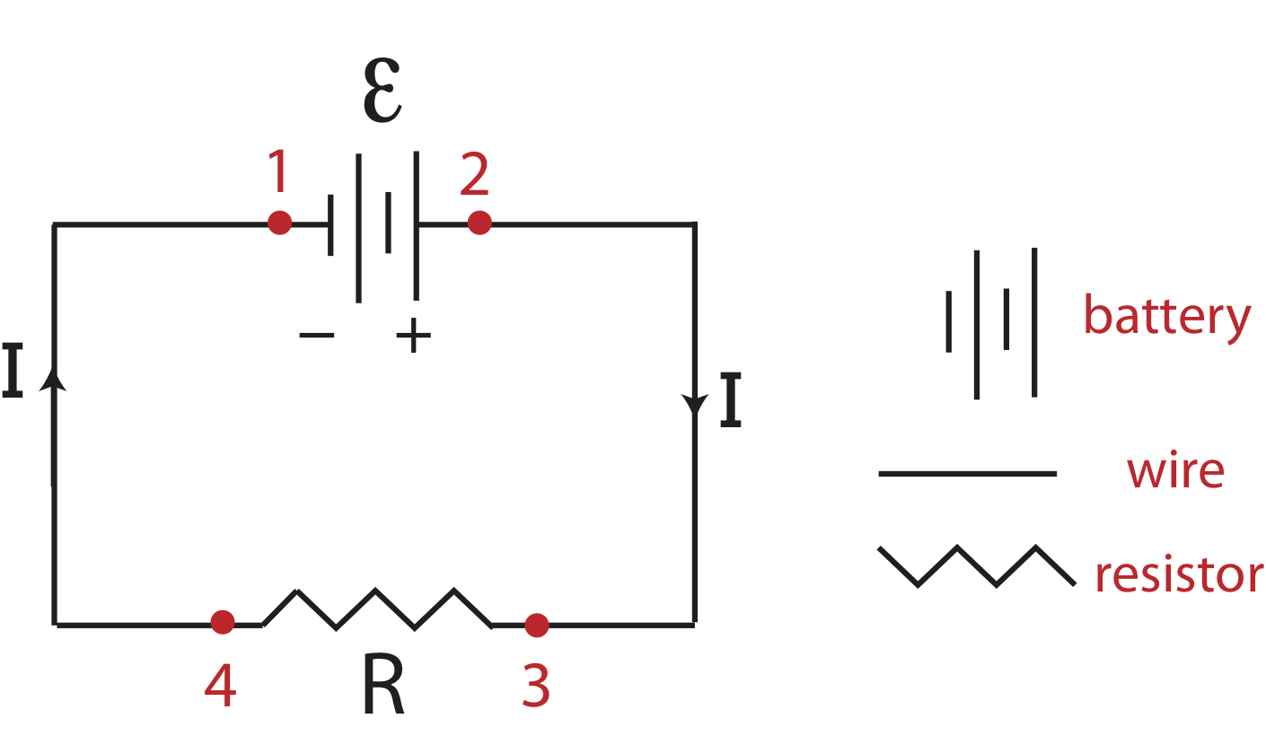
There is an important point we need to get very clear about right from the start. When charge flows in an electric circuit it is electrons, the negative charges, that flow from the negative terminal of the battery to the positive side in a counterclockwise direction in circuit in Figure 5.4.2. However, electric current is defined by convention as the flow of positive charge from the positive to the negative terminal of the battery, which is in the clockwise direction in Figure 5.4.2. Historically, positive charge was defined in a way that makes the charge on an electron negative. Now, when we speak of current as being in a particular direction, we mean positive charge flow. So, if that charge flow is due to the motion of electrons, then those electrons are in fact moving in the opposite direction. We will always emphasize charge flow, not the flow of the charge carriers, such as electrons, when using the steady-state energy-density model with electrical phenomena.

Electric current, \(I\), is the amount of charge that flows past a particular point per unit of time. Electric charge has units of coulombs, abbreviated \(C\). The unit of electric current is the ampere or amp for short, abbreviated with a uppercase letter "A", such that \(A \equiv C/s\). This is analogous to the volumetric flow rate which has units of volume per second, so it describes the amount of fluid flowing per unit time rather than the amount of charge flowing per unit time for charge flow.

The Complete Energy-Density Equation for Electric Circuits

In one way, current electricity is simpler than dissipative fluid flow. With fluids we have three energy-density systems that all contribute to the total head. In current electricity, there is only one energy system: the electric potential energy per charge. Since the mass of charge carriers and velocities are so small, both the gravitational potential energy and the kinetic energy changes are totally negligible compared to the changes in the electric potential energy. When dividing energy by electric charge, we turn the extensive electric potential energy, which depends on the amount of charge, into an intensive quantity. The electric potential energy per charge is given the name electric potential. Another common way to call the electric potential is voltage, which is what we will do from now on. Voltage has SI units of volts, abbreviated with uppercase "V". Since electric potential has units of energy per charge, a volt is a joule per coulomb, \(V=J/C\).

Batteries convert chemical energy (bond energy) into electric potential energy. Electromotive force, \(\mathcal E\) is an energy per charge and has units of volts, just like for electric potential. Common practice today is to speak of voltage instead of emf when referring to batteries and generators. Thus one commonly hears phrases such as, “The voltage of a ‘D' battery is 1.5 volts”.

Resistance to the flow of a fluid causes a transfer of energy from the fluid energy-density to thermal energy-density. Likewise, in electric circuits, resistance to the flow of charge causes transfer of electric potential energy to thermal energy-density. In both cases the amount of energy-density transferred is equal to the product of the current and the resistance. That is, \(\Delta E_{th}/C = IR\). The unit of electrical resistance is the ohm with abbreviation \(\Omega\). Using the four electric components just discussed, voltage, emf, current, and resistance, the complete energy-density equation for electric charge becomes:

\[\Delta V = \mathcal E – IR\label{circuit-full}\]

The meaning of Equation \ref{circuit-full} is completely analogous to the meaning of the complete energy-density Equation \ref{fluid-head} used for fluid flow phenomena. The arguments we made in developing the fluid version of the energy-density Equation \ref{fluid-head} apply to current electricity as well. If there are no sources or energy transfer into or out of the electric charge system, then the electric potential does not change. But if we attach batteries or generators, we put energy into the system. If there is a current and charge flows through conductors that have resistance, then electric potential energy per charge will be converted to thermal energy, which decreases the electric potential.

As with fluid circuits, we must always remember that the complete energy-density Equation \ref{circuit-full} applies to two specific points along the current path. The algebraic sign of the "IR" terms also works the same way. If we move in the direction of positive charge flow, i.e., in the direction of the current, then "IR" is positive, and the minus sign insures that voltage decreases in as we move in that direction. This is often referred to as a voltage drop, indicating that the value of \(\Delta V\) across a resistor in the direction of current is negative.

As we did with the fluid circuit, let us apply Equation \ref{circuit-full} across various points, 1-4, marked in Figure 5.4.2.

Across the battery:

\[V_2-V_1=\mathcal E\]

Across the wires:

\[V_3-V_2=0;~~~~V_1-V_4=0\]

Across the resistor:

\[V_4-V_3=-IR\]

When we add the four equation we find as we did for a fluid circuit, we find that the voltage around the circuit adds up to zero. If we add the right-hand sides of the 4 question and solve for current, we will get an equation analogous to Equation \ref{current-pump-R}:

\[I=\dfrac{\mathcal E}{R}\label{current-circuit}\]

The current in an electric circuit remains constant throughout the circuit since the flow is steady-state. But the magnitude of the current depends on the energy provided to the circuit by the battery and the amount of resistance present in the circuit. In the next section we will analyze circuits with more complex sets of resistors and batteries, but we will discover that all circuits can be reduced to the simplest circuit shown in  Figure 5.4.2, and Equation \ref{current-circuit} can be used to find the total current coming out of a battery in any circuit.

Power Relationships

The power relationships for current electricity are completely analogous to those for fluids shown in Section 5.3.

Rate of change of the electric potential energy:

\[P = |\Delta V| I \]

Rate energy is transferred into the electric potential by a battery or generator:

\[P = \mathcal E I \]

Rate energy is transferred into the thermal system from electric potential energy or voltage:

\[P = I^2R = \frac{( \Delta V)^2}{R}\]

Using dimensional analysis we can see that these equations give us units of power, \(W=J/s\).  Voltage has units of energy per charge, \(V=J/C\), and current is charge per using time, \(A=C/s\).  Multiplying units of voltage and current we find the units of power, \(J/s\).

 

Example \(\PageIndex{1}\)

Suppose a wire or a hose is carrying a steady-state current. The wire must be attached to batteries or other sources of emf, and be part of a larger closed circuit, but we will focus only on one segment of the circuit. Likewise, if this was a hose it would represent a section of a larger fluid system. We will not distinguish wires from resistors and will just assume that the wire has some internal resistance.  (The shape of section of wire or hose in the figure is meant to represent any general section of wire or hose. It continues in both directions.)

                                                        

a) Suppose the current in the wire is \(10 A\) and the resistance per meter of wire length is \(0.01 \Omega/m\). Find the voltage drop between points A and B, if the length of wire between points A and B is \(200 m\).

b) A voltmeter measures a voltage drop from B to C of -16 V. Find the resistance in segment BC.

c) Let us consider the analogous fluid example. Imagine that we now have a section of constant diameter fire hose carrying a current of \(1.0 \times 10^{-3} m^3/s\). The resistance per meter of length of hose is \(1.0\times 10^6 Js/m^7\). Find the drop in total head in going from A to B which is 200m long.

d) Is the change in pressure the same, greater, or smaller than the change in total head you found in part c)?

e) Find the power loss from A to B for both the wire and hose scenarios.

 

Solution

a) The resistance of the wire between points A and B is

\(R_{AB}=0.01 \dfrac{\Omega}{m}\times 200 m = 2\Omega\)

The voltage drop, \(\Delta V=-IR\) is:

\(\Delta V_{AB}=V_B-V_A=-IR_{AB}=-10A\times 2\Omega=-20V\)

b) The current is constant throughout the wire, so a smaller voltage drop implies a smaller resistance in the BC segment compared to AB segment.

\(R_{BC}=-\dfrac{\Delta V_{BC}}{I}=-\dfrac{-16 V}{10 A}=1.6\Omega\)

c) The resistance of the hose between points A and B is

\(R_{AB}=1.0\times 10^6 \dfrac{Js}{m^7}\times 200 m = 2.0\times 10^8\dfrac{Js}{m^6}\)

The total head change, \(\Delta \text{(total head)}=-IR\) is:

\(\Delta \text{(total head)}_{AB} = - 1.0\times 10^{-3} \dfrac{m^3}{s} \times 2.0\times 10^8\frac{Js}{m^6}= -2.0 \times 10^5 Pa= -2.0 atm\)

d) Total head represents the sum of changes in energy-densities. The hose has uniform area, so there is no change in kinetic energy-density between A and B.  However, point B is higher than point A, so there is an increase in gravitational potential energy:

\(\Delta\text{(total head)}_{AB} = \Delta P+\Delta PE_g= -2.0 atm\)

Since \(\Delta PE_g\) is positive, to get a negative change in total head the change in pressure must be negative as well and with a great magnitude than the change in total head. Thus, the change in pressure is greater than the change in total head.

e) The power loss of the electric charge or the fluid system from A to B is simply the product of the energy drop (voltage or total head) and the current:

electric: \(P=|\Delta V|I=20V\times 10A = 200 W\)

fluid: \(P=|\Delta\text{(total head)}|I=2.0\times 10^5 Pa\times 1.0\times 10^{-3} m^3/s =200W\)

Household Electricity

Utility companies such as PG&E and SMUD supply our workplaces and houses with alternating current (AC) electricity. The current varies sinusoidally, at 60 Hz, switching directions 120 times each second. The fundamental ideas we have developed to understand direct current (DC) circuits (as from a battery) can also be applied to AC sources. In fact, the values of the voltages and currents used when dealing with 60 Hz AC electricity are typically the root mean square values, which makes all the algebraic relationships we have developed applicable. Therefore, unless stated otherwise, values of voltages and currents for 60 Hz AC can be treated as DC values.

The primary reason AC is used in power distribution systems is the ease with which voltages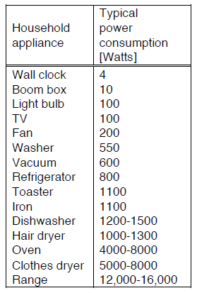 can be changed. The large round “cans” hanging on power poles are transformers. In a typical residential power distribution system, the wires at the top of the pole are often at 12,000 to 22,000 V. The transformer steps this voltage down to 120 V and 240 V, the voltage of wires entering most apartments and houses. We will study how transformers work in Physics 7C when we get into the fascinating world of the interaction of electricity and magnetism.

You probably use several small appliances everyday that make use of a “step-down” transformer. Many small computer peripherals have a small black box with two prongs sticking out that plugs into the 120 V power-outlet strip. The 120 V from the power strip is dropped down to 6 to 12 V in the isolation transformer. This is an excellent safety feature. Voltages in the 10 to 20 V range are relatively harmless to humans, if contact is limited to skin and not to internal organs. The 120 V in the wall outlet can cause sufficient currents through a person’s body when contact is made through skin and is definitely considered dangerous. The major health risk from 120 V shocks are currents in the chest region, which can cause the heart to go into fibrillation. Much larger currents cause burns, and ironically, can also be effective in stopping fibrillation of the heart. This is exactly what an AED, automated external defibrillator, does.

Every outlet in our homes can be considered a source of constant voltage of about 120 Volts. Each appliance has a characteristic resistance \(R\), and this determines how much power is used by this appliance when it is turned, using \(P = \dfrac{\Delta V^2}{R}\). The table on the rights gives some typical power values. When you pay your PG&E or SMUD electrical bill, they charge you for energy, not power. The unit they use, however, sounds like a power unit: kilowatt-hour. Can you explain why this is an energy unit?

Internal Resistance of Power Sources

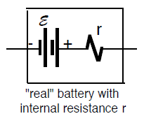Most wires used in house wiring, for appliances, and in lab, have very low resistance. In particular, the voltage drop across wire are small compared to other voltage changes in the circuits. Therefore, we typically model them as having zero resistance. Similarly, new batteries have resistance that are also small compared to the resistance of other components in the circuit to which the battery is attached. However, the internal resistance of batteries, labeled "r'" in the figure here, does increase over time, as the reactant chemicals inside turn into by-products that impede the flow of electrons through the battery. A 1.5V battery that is almost “used up” still provides charges that pass through it with almost 1.5 joules per coulomb. That is, it might still have an emf of nearly 1.5 V. But due to its high internal resistance r, most of this voltage is converted to thermal energy inside the battery itself when the battery is connected into a circuit. A battery that is very warm when it is being used is probably almost completely depleted.