3.3: Diffraction Gratings

Adding More Slits

After having determined the interference pattern associated with two slits, it makes one wonder what would happen if many more (equally-spaced) slits are added. We can recycle our geometrical analysis from the double slit problem to answer this question. Let's look at the example of four slits.

We begin once again with the assumption that the distance to the screen is significantly larger than the separation of adjacent slits: \(d\ll L\)). Starting with the lowest slit of the four as a "reference" and repeating the double-slit geometry for each slit going up from there, we have a diagram that looks like this:

Figure 3.3.1 - Geometry of Four Slits

The \(\Delta x\) in each case is the difference in distance traveled compared to the reference slit. So the extra distance traveled by the wave following the blue path is three times as great as the extra distance traveled by the wave following the orange path.

Alert

This diagram is blown-up for clarity, but doing so makes the angles quite different from each other. With the proper scale in place the approximations of equal angles (and equal ∆x’s throughout) would be more apparent.

Okay, so as our first task, we will look for the position where the first bright fringe is located. For this to occur, we need all four waves to be in phase, which means that \(\Delta x\) has to be a full wavelength, giving us the same formula for bright fringes that we found for the double slit:

\[d\sin\theta=m\lambda\;,\;\;\;\;\;m=0,\;\pm1,\;\pm2,\;\dots\]

[It should be noted that the positions of the fringes on the screen are measured from the horizontal line passing through the center of the collection of slits, as we did with the double slit.]

Does this mean that the result for several slits is identical to that of the double slit? Certainly not! First of all, there are many more sources of light, all interfering constructively, which means that the bright fringes are much brighter. How much brighter? Well, with four slits, as in the example here, the amplitude of a single slit is multiplied by 4, making the intensity (which goes as the square of the amplitude) 16 times greater than a single slit. For the double slit, the intensity was increased by a factor of 4 (the amplitude was doubled). Therefore doubling the number of slits increased the intensity of the bright fringes by a factor of 4. But wait, doubling the number of slits only lets in twice as much energy per second, so how is the intensity increasing so much?

The answer to this puzzle involves how concentrated the bright fringes are. All bright fringes have a point of maximum brightness that tapers down to the dark fringes. If the rate at which the brightness tapers down is greater, then the brightness (energy density) near those maximum points can go up, and the energy density near the dark fringes goes down, such that the same total energy hits the screen. But it turns out there is even a little more to it than this, as we will now see.

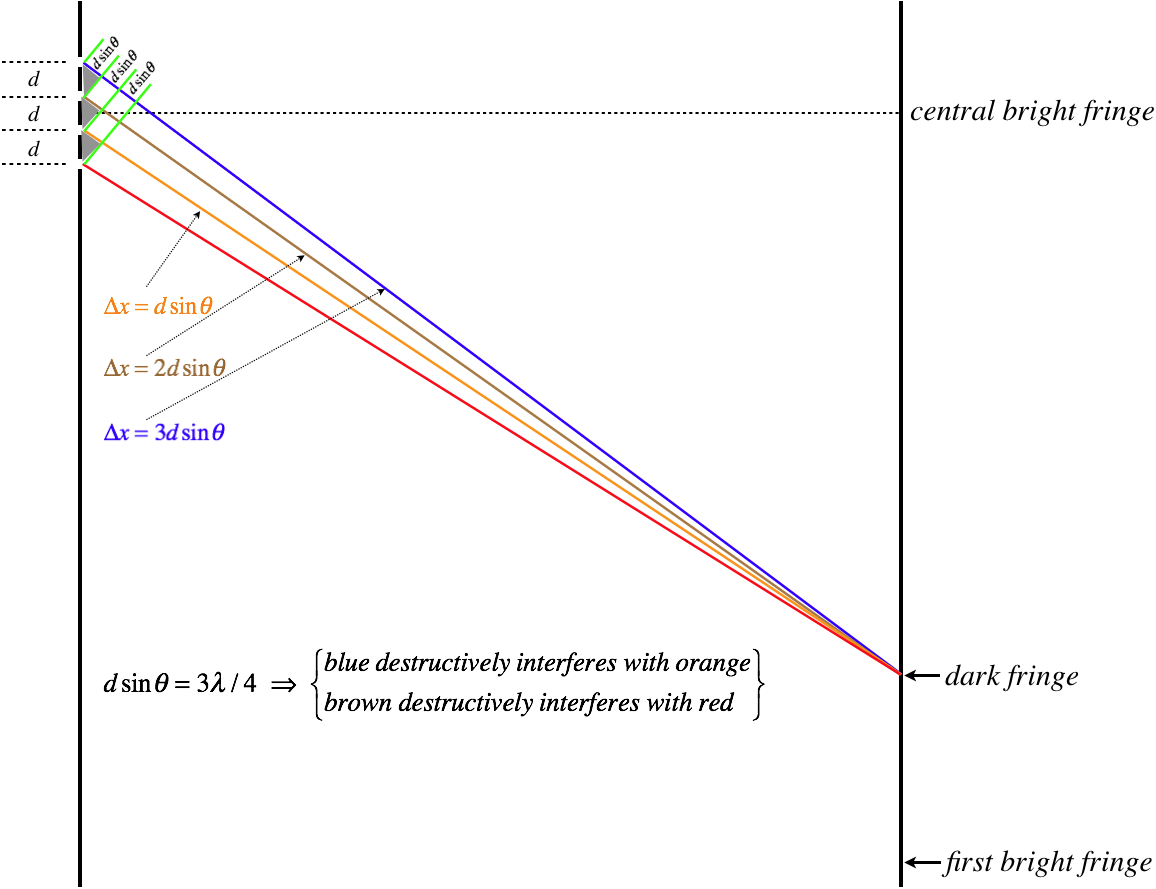
To demonstrate this phenomenon, it becomes necessary to redraw the figure above a little closer to the actual scale. We of course cannot possibly get very close to the actual scale, as slit separations are typically fractions of millimeters, while distances to screens are usually tens or hundreds of centimeters, but we will use what space we can manage. As before, we will use the red line as the reference, and compare the distances traveled by the other three light waves.

Figure 3.3.2a - Finding Dark Fringes

We'll start with the bright fringe, and start working our way closer to the central bright fringe until we hit a dark fringe. Strangely, we find that the first position of total destructive interference we encounter does not occur at the halfway point, as it did for the double slit! Note that when the distance \(\Delta x=d\sin\theta\) equals three-quarters of a wavelength, then the wave that follows the blue path will travel 1.5 wavelengths farther than the wave that follows the the orange path, and as this is an odd number of half wavelengths, these waves will cancel. The same is true for the waves that follow the brown and red paths, which means that position will be completely dark.

Figure 3.3.2b - Finding Dark Fringes

So what happens if we keep going up the screen? We don't find any more maximally-bright fringes (all four waves can't be in phase), but we do find another totally dark position. It occurs when the distance \(\Delta x=d\sin\theta\) equals one-half of a wavelength. In this case, The wave that follows the blue path travels one half-wavelength farther than the wave that follows the brown path, and the waves that follow the orange and red paths also differ in the distance they travel by one half wavelength. So the blue path and red path waves cancel, as do the brown path and yellow path waves, resulting in total darkness.

Figure 3.3.2c - Finding Dark Fringes

There is one other time when a dark fringe occurs. This happens when the distance \(\Delta x=d\sin\theta\) equals one-quarter of a wavelength. Once again, alternate slits interfere with each other, as the waves travel distances that differ by a half-wavelength.

We can also show this phenomenon mathematically, by superposing (adding) the wave functions. The waves start in phase at the slits, so all of the phase constants are equal (and we choose them to be zero at \(t=0\)), so all that remains of the wave functions is the position dependence. Once again, all that matters are the differences in distances traveled with the reference slit (whose difference with itself is zero), so the superposition intensity looks like:

\[\begin{array}{l} I_\text{2 slits}\left(\theta\right) && = && \left\{f_1\left(\theta\right)+f_2\left(\theta\right)\right\}^2 && = && \left\{\cos 0+ \cos\left[ \left(\frac{2\pi}{\lambda}\right)d\sin\theta\right]\right\}^2 \\ I_\text{3 slits}\left(\theta\right) && = && \left\{f_1\left(\theta\right)+f_2\left(\theta\right)+f_3\left(\theta\right)\right\}^2 && = && \left\{\cos 0+ \cos \left[\left(\frac{2\pi}{\lambda}\right)d\sin\theta\right]+ \cos \left[\left(\frac{2\pi}{\lambda}\right)2d\sin\theta\right]\right\}^2 \\ I_\text{4 slits}\left(\theta\right) && = && \left\{f_1\left(\theta\right)+f_2\left(\theta\right)+f_3\left(\theta\right)+f_4\left(\theta\right)\right\}^2 && = && \left\{\cos 0+ \cos \left[\left(\frac{2\pi}{\lambda}\right)d\sin\theta\right]+ \cos \left[\left(\frac{2\pi}{\lambda}\right)2d\sin\theta\right]+ \cos \left[\left(\frac{2\pi}{\lambda}\right)3d\sin\theta\right]\right\}^2 \\ I_{n\text{ slits}}\left(\theta\right) && = && \left\{f_1\left(\theta\right)+f_2\left(\theta\right)+\dots + f_n\left(\theta\right)\right\}^2 && = && \left\{\cos 0+ \cos \left[\left(\frac{2\pi}{\lambda}\right)d\sin\theta\right]+\dots + \cos \left[\left(\frac{2\pi}{\lambda}\right)\left(n-1\right)d\sin\theta\right]\right\}^2\end{array}\]

Putting these functions into a graphing calculator confirms what we found above, as well as what we suspect about \(n\) slits – that there are \(n-1\) dark fringes between each maximally-bright fringe.

Figure 3.3.3 - Comparison of Interference Patterns by Number of Slits

Notice that the bright fringes for any number of slits occur at the same places as for the double slit (provided they have the same slit separation), and that the number of dark fringes between bright fringes goes up by one every time another slit is added. Also notice that the maximum intensity of the double slit is 4 units, the 3-slit case has a maximum intensity of 9 units, and for 4-slits it is 16 units, as we expect when the amplitude increases by one unit with the addition of each slit. But also notice that the widths of the bright fringes get narrower, indicating that the energy becomes more concentrated near the brightness maxima, and less concentrated near the dark fringes.

It turns out that we can mathematically check that the energy is in fact conserved by this mechanism. Recall that the intensity is related to power density, which means that if we integrate one of these curves over a full interval of space that the light is landing (say, between adjacent bright maxima), we get a measure of the energy landing in that region per unit time. Once again the graphing calculator comes in handy (unless integrating the intensity functions above is your idea of fun) as areas under these curves between maxima come out to be in relative proportions of 2:3:4 – the total energy landing on the screen every second really is proportional to the number of slits allowing light through!

Adding Many, Many More Slits

We know that the regions where the bright fringes peak get more concentrated light, and that there are more dark fringes between them when the number of slits is increased. One can imagine that in the limit where very many slits are used (a device called a diffraction grating), the result is very sharp, very bright lines lines at the points of maximum constructive interference, and darkness everywhere else. As we will see, this will be an extremely useful feature. But there is one assumption we have made here that needs to be emphasized. Because \(d\) is so small compared to the distance to the screen, it was easy to ignore the fact that this particular calculation required the assumption that the first bright fringe be farther from the center line than the outermost slit (we assumed that the wavelength was long enough that this had to be true). So creating a sharper interference pattern for a given wavelength of light by adding more slits at the same separation on both sides of the center line has limitations, because when the number of slits gets very large, the added slits go past the bright fringe. However, if more slits are added by squeezing them closer together (making \(d\) smaller), then for a given wavelength, then not only are there more slits, but the angle to the first bright fringe increases, thanks to the relation \(d\sin\theta=m\lambda\).

It is for this reason that diffraction gratings are generally characterized by their grating density – the number of slits per unit distance. Of course such a number can be converted into a slit separation: If a diffraction grating has a grating density of 100 slits per \(cm\), then the slits must be separated by \(d=\frac{1}{100}cm = 10^{-4}m\). This number can then be used in calculations for the angle at which bright fringes are seen.

It should also be mentioned that like double slits, diffraction gratings do allow for more than one bright fringe (as before, depending upon the ratio of \(d\) and \(\lambda\)). For a typical double slit experiment, the goal is usually to show a broad interference pattern – many fringes. If the slit separation is too small, then the angles between the fringes are large, resulting in very few fringes, widely separated, foiling the goal of such an experiment. But use of a diffraction grating has a different goal (very sharp bright fringes), which requires that the slits be separated by much smaller distances. This results in far fewer fringes, separated by large angles. So while the calculation for the angles of bright fringes is the same for both devices, for a given range of wavelengths, their slit separations are usually quite different.

Applications of Diffraction Gratings

It was stated above that sharp bright fringes are very useful in applications. To see why this is so, suppose one wishes to use a diffraction device to measure the wavelength of a monochromatic light. This is straightforward – shine the light through any number of slits with a known slit spacing, and measure the angle at which the first bright fringe is deflected from the central bright fringe, then plug into \(d\sin\theta=m\lambda\) (with \(m=1\)) and solve for \(\lambda\). The only real challenge to this procedure is measuring the angle. Of course, if we shine the light onto a screen whose distance we know from the slits, we can measure the distances between the bright fringes, and compute the angle from there. But still we have a problem if we want to be precise. If a double-slit is used, then the bright fringe is rather broad, and it might be challenging to get a good measurement of its center. With a diffraction grating, the bright fringe is much better defined. Furthermore, the light we are looking at may not be very intense, and a diffraction crating lets much more of the light in, and the bright fringe is much easier to see than it would be for a double-slit.

But even these two advantages pale in comparison to the third. We have not yet considered what happens if we look at light that is not monochromatic. Suppose the incoming light is a mix of three or four colors. The separate colors don't interfere in a static manner with each other (they can create "beats," but the frequency differences for light are so great that these will not be observable) they only observably interfere with themselves. As such, a beam of light with three colors will exhibit three separate interference patterns when passed though a single device (i.e. they all experience the same slit separation). The wave with color corresponding to the shortest wavelength will have its first bright fringe deflected by the smallest angle. If this light is passed through a double-slit, the interference patterns blend with each other, making it hard to separate the component colors. But a diffraction grating makes three sharp, distinct, first-order bright fringes, making it easy to determine the constituent colors of the incoming light.

An important part of the fields of chemistry and astronomy is the method of measurement called spectroscopy. In Physics 9D, you will learn that matter emits and absorbs light in very peculiar ways. You might think that electrons in atoms can vibrate at any frequency at all and therefore emit or absorb a nice, smooth continuous spectrum of light, but it turns out that they cannot. In fact each atom has a unique “fingerprint” of specific frequencies of light that it emits and absorbs. This means that when light emitted from a certain substance is passed through a diffraction grating, this fingerprint is manifested as a specific set of bright fringes (called spectral lines). This means that we can ascertain from a distance (in the case of astronomy, very great distances!) the composition of the matter that is emitting light. These fingerprints are so specific and unique that even if several different substances are emitting light, they can generally be sorted out.

One might worry that since stars are moving relative to the earth, that we might get the elements wrong, since what we will see in the spectrometer (a device with a diffraction grating) will measure doppler-shifted wavelengths. But it isn't the exact positions of the spectral lines that tells us the elements emitting the line, but rather their relative positions. That is, every spectral line is doppler-shifted, so the "barcode" essentially looks the same for hydrogen regardless of its relative motion, because the whole barcode is just shifted toward longer wavelengths if it is moving away from the spectrometer, and toward the shorter wavelengths if moving toward the spectrometer.

But astronomers can do even more than identify elements in burning stars. We know what the barcode for hydrogen looks like when the source is at rest relative to the spectrometer, so when we see the hydrogen barcode pop up for a star, we can measure how much the barcode in the spectrometer is shifted compared to the stationary case, and we can use the amount of shift to determine how fast the star is moving relative to earth!

Example \(\PageIndex{1}\)

A spaceship is fitted with a light beacon before blast-off. The light from this beacon is monochromatic, and when it is shone through the apparatus pictured below, the angle of deflection of the first order bright fringe is measured. The spaceship then blasts off, and after several years of accelerating through outer space, it is moving away from the Earth at a very high rate of speed, and the light from its beacon is shone through the apparatus again (which is still on Earth).

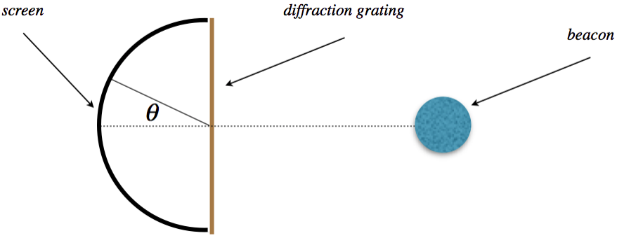
1. Will the angle of deflection of the first-order bright fringe for the beacon coming from the moving ship be greater or less than the angle measured before blast-off? Explain.
2. Suppose deflection angle of the first order bright fringe changes by 10% as a result of the spaceship’s motion (so it is either 90% or 110% of what it was before, depending upon your answer above). Find the speed of the spaceship. Assume that the deflection angle is small, so that sine of the angle changes by the same percentage as the angle itself when measured in radians.

Solution

a. The ship is receding, so the source of the light is moving away from the receiver. This doppler-shifts the light to a lower frequency, which corresponds to a longer wavelength. The relationship between the angle of the first bright fringe and the wavelength is:

\[d\sin\theta = m\lambda \;\;\;\Rightarrow\;\;\; \sin\theta = \frac{\lambda}{d} \nonumber\]

The separation of the slits doesn’t change, so as the wavelength gets longer, the sine of the deflection angle gets bigger, which means the angle itself gets bigger.

b. From our answer above, the deflection angle has grown to 110% of what it was before blastoff. By our small-angle approximation, we can therefore say that the sine of the angle has grown by the same amount, which means that is how much the wavelength has shifted longer. The doppler shift formula (for light) gives a relationship between the sender’s frequency and the receiver’s frequency when the two are moving away from each other, and we can turn this into a relation between the wavelengths using Equation 2.2.10:

\[f_r = \sqrt{\dfrac{c-v}{c+v}} f_s \;\;\;\Rightarrow\;\;\; \dfrac{c}{\lambda_r} = \sqrt{\dfrac{c-v}{c+v}} \dfrac{c}{\lambda_s} \;\;\;\Rightarrow\;\;\; \dfrac{\lambda_r}{\lambda_s} = \sqrt{\dfrac{c+v}{c-v}} \nonumber\]

We found that the received wavelength is 10% longer than the sent wavelength, which means that the ratio of these wavelengths is 1.1. Plugging this in allows us to solve for the velocity of the source (i.e. the ship):

\[1.1 = \sqrt{\dfrac{c+v}{c-v}} \;\;\;\Rightarrow\;\;\; 1.21 \left(c-v\right)= \left(c+v\right) \;\;\;\Rightarrow\;\;\; v = \dfrac{0.21}{2.21}c = 2.9\times 10^7\frac{m}{s} \nonumber\]