3.5: RC Circuits

Capacitors in Networks

We can see how Kirchhoff’s rules helps us analyze circuits that either involve awkward combinations of resistors or multiple batteries, but what about including capacitors along with those components? Let’s look at a sample of such a network.

Figure 3.5.1 – A Sample Network involving Resistors and Capacitors

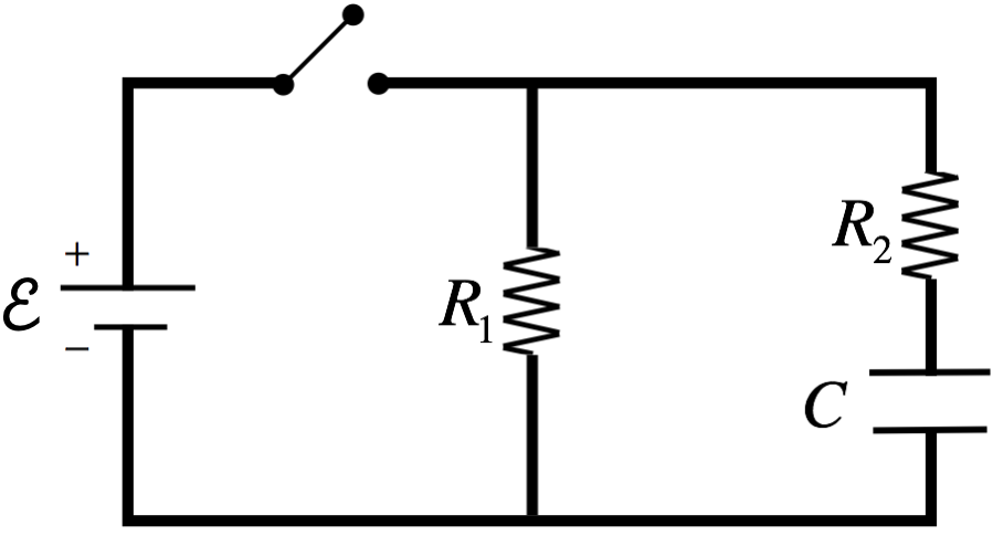
The question we want to answer is the usual: "After the switch is closed, what is the current through each resistor?" To answer this question, we start by invoking Kirchhoff's loop rule around the outside loop (clockwise, starting in the lower left corner), and noting that the potential difference between two plates of a capacitor is the ratio of the charge and capacitance, we get:

\[+\mathcal E -I_2R_2 - \dfrac{Q}{C} = 0\]

So in order to ascertain the value of \(I_2\), we need to know how much charge is on the capacitor. Given that charge that flows through the resistor \(R_2\) will be deposited on the plates of the capacitor, it's clear that the amount of charge on the capacitor changes over time. The emf provided by the battery is steady, so this means that the current through the resistor depends upon how much charge started on the capacitor, and how long the switch has been closed. Let's look at two special cases, both of which involve the capacitor being uncharged when the switch is closed.

no initial charge on capacitor, just after the switch is closed

At the moment when the switch is closed, there has not yet been any time for charge to accumulate on the capacitor. With zero charge on it, the voltage difference between the plates is zero. Plugging this into the loop equation above reveals that the current through the resistor is exactly what it would be if the capacitor were not even present. This will of course not remain the case, as the capacitor will begin charging, but at the moment when the current starts, the capacitor can simply be ignored. This result is not special to this particular network – it is generally true, no matter how complicated the network might be:

A capacitor that contains zero charge at an instant in time can be treated as an equipotential within the network at that moment.

capacitor fully charged, a long time after the switch is closed

When the capacitor has been allowed to charge a long time, it will become "full," meaning that the potential difference created by the accrued charge balances the applied potential. In this case, the first and third terms of the Kirchhoff loop equation for the outer loop cancel, which means that no current passes through resistor \(R_2\). In a direct current network, the charge can only accumulate on a capacitor (it doesn't come back off), so it doesn't matter how complicated the network is, given a long enough period of time, the capacitor will fill, and will stop all the current flowing through that branch from flowing.

A capacitor that has spent a long time in a closed network will be fully charged, and will not allow any current to pass through the branch it occupies, so it can be treated as if it is an open switch.

You may be wondering how a capacitor (which provides a gap in the conductor) is different from simply a break in the wire. That is, we know that if we cut the wire, the light bulb goes out immediately, while a capacitor allows it to shine (until it is fully charged). The answer is that they are in fact the same! Think about the capacitor that cutting a wire creates: It is the thickness of the wire (very thin), and is typically separated by a very large distance. Using the parallel-plate case as a model, this results in a very small capacitance, which means that for the voltage supplied the amount of charge required to “fully charge” it is very small. The current will not take long at all to do this, so the light shines for only an extremely short time. In the limit where we treat “cutting the wire” as completely disassociating the two open ends, there is zero capacitance, which means zero charge, which means no current through the resistor at all.

A Discharging Capacitor

Now we need to figure out what happens during the time period when a capacitor is charging. We start with the most basic case – a capacitor that is discharging by sending its charge through a resistor. We actually mentioned this case back when we first discussed emf. As we said then, the capacitor can drive a current, but as the charge on the capacitor neutralizes itself, the current will diminish.

Figure 3.5.2 – A Discharging Capacitor

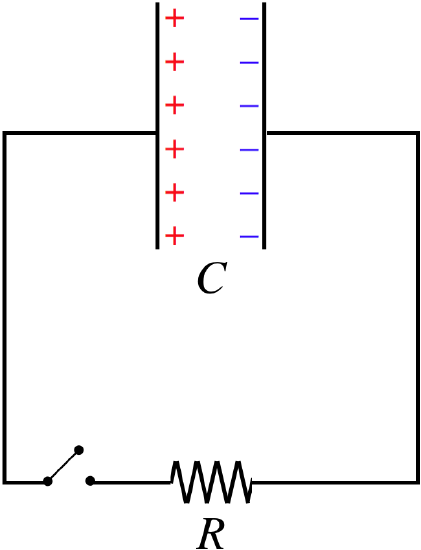
We will assume that the capacitor starts with a charge equal to \(Q_o\). We seek to determine everything there is to know about the circuit (charge on the capacitor \(Q\), current through the resistor \(I\), etc.) at a time \(t\) if the switch is closed at time \(t=0\). Start by using Kirchhoff's loop rule to relate the voltage differences across the two components at some arbitrary time \(t\). Let's label the current so that it is going in the direction we know it must go (counterclockwise), and choose our loop direction the same way. Then starting in the upper-right corner, we see that when we jump across the capacitor we see an increase in potential equal to the voltage across the capacitor, and a decrease in potential across the resistor (because the loop direction matches the labeled current direction).

\[+\dfrac{Q}{C} - IR = 0 \;\;\;\Rightarrow\;\;\; I = \dfrac{1}{RC} Q\left(t\right)\]

Now we need to relate the current through the resistor to the charge on the capacitor. Clearly the current is the rate at which charge is leaving the capacitor, which means \(I = \left|\frac{dQ}{dt}\right|\), but what should the sign be? Well, since \(Q\left(t\right)\) is getting smaller as the current flows in the direction we selected, it must be that a positive current equals the negative of the rate of change of the charge on the capacitor. Plugging this in gives:

\[-\dfrac{dQ}{dt} = \dfrac{1}{RC} Q\left(t\right)\]

This leaves us with a differential equation that is not difficult to solve. Isolate the variable \(Q\) on the left and the variable \(t\) on the right, and integrate:

\[-\int\dfrac{dQ}{Q} = \int\dfrac{dt}{RC} \;\;\; \Rightarrow \;\;\; -\ln Q = \dfrac{t}{RC}+const \;\;\; \Rightarrow \;\;\; Q\left(t\right) = Q_oe^{-\frac{t}{RC}}\]

The final step perhaps requires come clarification. In clearing the natural logarithm function, the additive constant term becomes a multiplicative constant term. To determine what this constant is, we plug in \(t=0\) (turning the exponential into a 1) and set \(Q\left(t=0\right)\) equal to the charge that the capacitor started with, which we defined to be \(Q_o\).

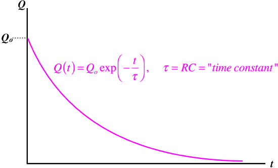
We therefore find that the charge on the capacitor experiences exponential decay. The rate of the decay is governed by the factor of \(RC\) in the denominator of the exponential. This value is called the time constant of that circuit, and is often designated with the Greek letter \(\tau\).

Figure 3.5.3 – Exponential Decay of Charge from Capacitor

Digression: Half-Life

The differential equation that led to the exponential decay behavior for the charge on a capacitor arises in many other areas of physics, such as a fluid transferring through a pipe from one reservoir to another, and nuclear decay. A common way to express the time constant of such a system is in terms of a quantity known as half-life. This is defined as the period of time that must pass for a system to lose half of whatever is decaying (such as the capacitor losing half its charge). It is easy to compute in terms of the time constant:

\[Q\left(t\right) = \frac{1}{2}Q_o = Q_o e^{-\frac{t_{1/2}}{\tau}} \;\;\; \Rightarrow \;\;\; t_{1/2} = \tau\ln 2 \nonumber\]

It is interesting to note that the half-life is the same period of time, no matter what the starting value of the decaying quantity is. So if the charge on a capacitor starts at \(Q_o\) and decays for a half-life, then it's new charge is \(\frac{Q_o}{2}\), and if it further decays from there for another half-life, then the charge drops to \(\frac{Q_o}{4}\).

We can also look at what happens to the current in a discharging capacitor. We already have the relationship between the current and the charge on the capacitor, so it's simple to write down:

\[I\left(t\right) = \dfrac{1}{RC} Q\left(t\right) = \dfrac{Q_o}{RC}e^{-\frac{t}{RC}} =I_oe^{-\frac{t}{RC}}\]

In the final step we used the zero voltage drop around the loop at \(t = 0\) to replace the combination of constants with the initial current. We see that the current also dies-off exponentially.

One last thing we can look at is the power dissipation. Energy is clearly leaving the capacitor as it charge drops, and energy is leaving the circuit as it is being converted to thermal by the resistor. These rates need to be equal (otherwise, where else is the energy going?), and we see that this is the case:

\[\begin{array}{l} \dfrac{dU}{dt} = \dfrac{d}{dt} \left[\dfrac{Q^2}{2C}\right] = \dfrac{1}{2C}\dfrac{d}{dt}\left[Q^2\right] = \dfrac{1}{2C}\left[2Q\dfrac{dQ}{dt}\right] = \dfrac{1}{C}\left[Q_oe^{-\frac{t}{RC}}\right]\left[-\dfrac{Q_o}{RC}e^{-\frac{t}{RC}}\right]=-\dfrac{Q^2_o}{RC^2}e^{-2\frac{t}{RC}} \\ P = -I^2R = \left[I_oe^{-\frac{t}{RC}}\right]^2R = -I^2_oR\;e^{-2\frac{t}{RC}} = -\dfrac{Q^2_o}{RC^2}e^{-2\frac{t}{RC}}\end{array}\]

Example \(\PageIndex{1}\)

The parallel-plate capacitor in the circuit shown is charged and then the switch is closed. At the instant the switch is closed, the current measured through the ammeter is \(I_o\). After a time of \(2.4s\) elapses, the current through the ammeter is measured to be \(0.60I_o\), and the switch is opened. A substance with a dielectric constant of 1.5 is then inserted between the plates of the capacitor, and the switch is once again closed and not reopened until the ammeter reads zero current.

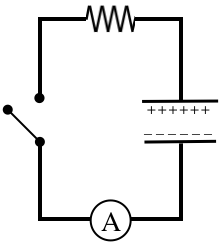
1. Find the period of time that elapses between when the switch is closed the second time and when the ammeter reads a current of \(0.20I\).
2. At the end, all of the electrical potential energy is gone from the capacitor. Find the fraction of this energy that was converted into thermal energy by the resistor.

Solution

a. We can calculate the time constant from the period of time that the current takes to drop to 0.6 of its original value:

\[0.60I_o = I_oe^{-\frac{t}{\tau}}\;\;\;\Rightarrow\;\;\; \tau = \dfrac{-t}{\ln0.60} = \dfrac{-2.4s}{\ln0.60} = 4.7s\nonumber\]

When the dielectric is inserted, the time constant changes. The time constant is proportional to the capacitance, so since inserting the dielectric increases the capacitance by a factor of 1.5, that is the factor by which the time constant changes as well, giving a new time constant of:

\[\tau = RC \;\;\;\Rightarrow\;\;\; \tau_{new} = R\left(\kappa C\right) = \kappa\tau_{old} = \left(1.5\right)\left(4.7s\right) = 7.0s\nonumber\]

The current is driven by the potential difference across the capacitor, and this is proportional to the charge on the capacitor, so when the current gets down to 60% of its initial value, that means that the charge on the capacitor has dropped by the same factor. To find the time for the current to drop to \(0.20I_o\), we need to know not only the new time constant, but also the new starting current. We can get this from the new starting voltage, which comes from the new starting charge and capacitance:

\[V_{o(new)} = \dfrac{Q_{o(new)}}{C_{new}}\;\;\;\Rightarrow\;\;\; I_{o(new)}\dfrac{V_{o(new)}}{R} = \dfrac{Q_{o(new)}}{RC_{new}} = \dfrac{0.60Q_o}{R\left(1.5C\right)} = 0.40I_o\nonumber\]

With the new starting current equal to \(0.4I_o\), we are looking for the time it takes to get down to \(0.2I_o\), so:

\[0.20I_o = 0.40I_oe^{\frac{t}{\tau}} \;\;\;\Rightarrow\;\;\; t = \tau\ln 2 = \left(7.0s\right)\ln 2 = 4.8s \nonumber\]

b. We already determined that in the first stage of this process, the charge on the capacitor went down to 60% of its initial amount. This allows us to calculate the energy lost by the capacitor, which is what is converted to thermal:

\[\Delta U_1 = U_o - \dfrac{\left(0.60Q_o\right)^2}{2C} = U_o - 0.36\dfrac{Q_o^2}{2C}=0.64U_o \nonumber\]

So 64% of the energy on the capacitor is converted to thermal energy in the first stage. In the second stage, all of the internal energy in the capacitor is converted, but this amount of energy must be calculated in terms of the new capacitance:

\[\Delta U_2 = \dfrac{\left(0.60Q_o\right)^2}{2\left(1.5C\right)} = 0.24U_o \nonumber\]

So of the original energy stored in the capacitor, 88% of the energy is converted to thermal. Where is the remaining 12%, if all of it is now gone from the capacitor? The field of the capacitor did work drawing the dielectric into it.

A Charging Capacitor

The case of a charging capacitor is not much different, though there are a few nuances to look at. We follow the same procedure as above, starting with the Kirchhoff loop.

Figure 3.5.4 – Charging Capacitor, Initially Uncharged

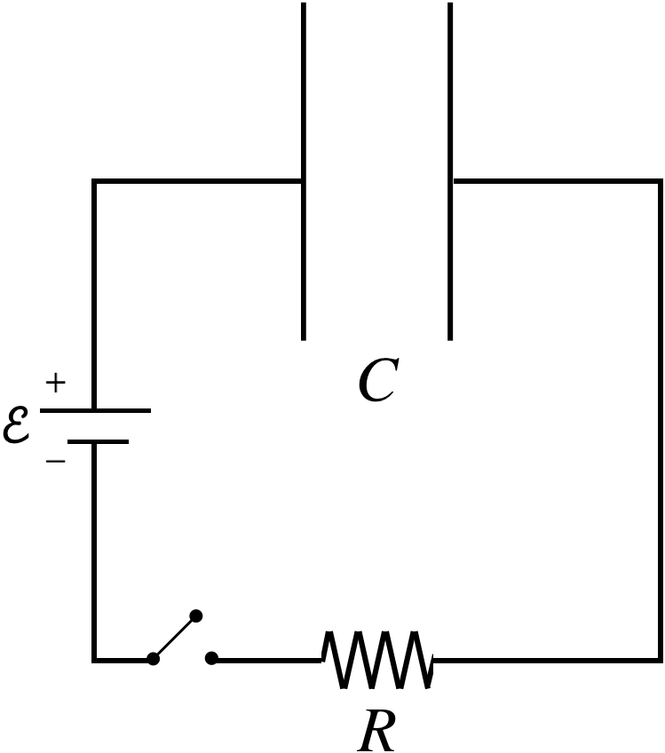
This time there is a battery included, and the positive lead of the battery charges the positive plate of the capacitor, so following the loop clockwise, with the current defined tin the same direction, and starting in the lower-left corner, results in an increase in potential across the battery, a decrease across the capacitor (goes from positive plate to negative plate), and a decrease across the resistor (in the direction of the current):

\[+\mathcal E -\dfrac{Q}{C} -IR =0\]

This time the positive current results in an increase to the charge on the capacitor, so the current is related to the charge as the positive derivative, giving us the differential equation:

\[+\mathcal E -\dfrac{Q}{C} -\dfrac{dQ}{dt}R =0\;\;\;\Rightarrow\;\;\; \dfrac{dQ}{dt} = \dfrac{\mathcal E}{R} - \dfrac{Q}{RC}\]

Isolating the \(Q\) and \(t\) variables and integrating:

\[\int\dfrac{dQ}{Q-\mathcal EC} =-\int\dfrac{dt}{RC}\;\;\;\Rightarrow\;\;\; \ln\left[Q-\mathcal EC\right] = -\dfrac{t}{RC}+const\]

As before, we find the integration constant by plugging in \(t=0\). This time the starting charge is zero, so:

\[const = \ln\left[-\mathcal EC\right] \;\;\;\Rightarrow\;\;\; -\dfrac{t}{RC} = \ln\left[Q-\mathcal EC\right]-\ln\left[-\mathcal EC\right] = \ln\left[\dfrac{Q-\mathcal EC}{-\mathcal EC}\right] = \ln\left[1-\dfrac{Q}{\mathcal EC}\right]\]

Solving for \(Q\left(t\right)\) gives:

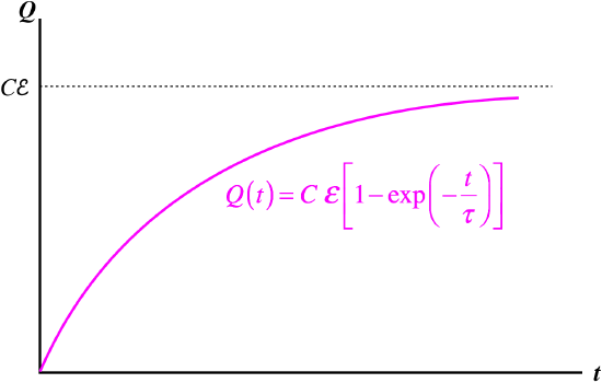
\[Q\left(t\right) = C\mathcal E \left[1-e^{-\frac{t}{RC}}\right]\]

So we see the exponential function again making an appearance, but this time it results in the charge asymptotically approaching its maximum (when the capacitor is fully-charged and has a potential across it equal to the battery). The time constant for this is the same as in the discharging case.

Figure 3.5.5 – Charge on Capacitor Asymptotically Approaches a Maximum

The current as a function of time turns out to be identical to that of the discharging capacitor, since the derivative of the constant term in the charging case is zero. That is, the current exponentially decays in both cases, as the system evolves toward equilibrium.

The fate of the energy of this system is a bit more interesting than is was in the obvious case of the discharging capacitor, when all the energy in the capacitor was converted to thermal energy. Here the battery is supplying energy, some of which is lost to thermal energy, and rest is stored in the capacitor. It is interesting to ask how much of the energy goes to each, and the answer is somewhat surprising.

We start by computing the total energy supplied by the battery. We know the power supplied by the battery is its voltage multiplied by the current, so we can write down the power supplied as a function of time:

\[P_{battery} = \mathcal E I = \mathcal E I_o e^{-\frac{t}{RC}} \]

But we are interested in the total energy supplied over the entire period of time that current is flowing, which means that we need to integrate this power function from \(t=0\) to \(t=\infty\):

\[U_{battery} = \mathcal E I_o \int\limits_0^{\infty} e^{-\frac{t}{RC}}dt =-\mathcal E I_oRC \left[e^{-\frac{t}{RC}}\right]_0^\infty = \mathcal E I_oRC\]

When the switch is first closed, it is as though the capacitor isn't there, so the initial current multiplied by the resistance is the voltage drop across the resister at that moment, which is simply the emf supplied by the battery, giving us:

\[U_{battery} = C\mathcal E^2\]

We know that at the end, the capacitor is fully-charged, and therefore is at the same voltage difference as the battery, giving it a total stored energy equal to:

\[U_{capacitor} = \frac{1}{2}C\mathcal E^2\]

So we see that exactly half the energy that comes from the battery goes to the capacitor, which means that the other half is converted to thermal energy by the resistor.

Example \(\PageIndex{2}\)

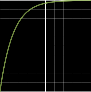
A voltmeter that plots potential differences in real time is connected across the plates of a capacitor as it is charged in a simple circuit that includes the capacitor (which starts with zero charge), a battery, and a resistor all in series. The voltmeter's output is shown below, with each marking along the horizontal axis representing 2 milliseconds and each marking along the vertical axis representing 1 volt. An ohmmeter used to measure the resistance in the circuit gives it to be \(1500\;\Omega\).

1. Find emf of the charging battery.
2. Find the capacitance of the capacitor.

Solution

a. The capacitor starts at zero potential difference (it is uncharged), and asymptotically approaches a potential difference of \(10V\). The capacitor stops charging when it reaches the emf of the battery, so the battery's emf is \(10V\).

b. We know the resistance of the circuit, so if we can determine the time constant of the circuit, we can compute the capacitance. This capacitor reaches half its charge after \(2\;ms\) (one horizontal grid line), so this gives us all we need to compute the time constant:

\[\frac{1}{2}Q_o = Q_o\left(1-e^{-\frac{2\;ms}{\tau}}\right) \;\;\;\Rightarrow\;\;\; \tau = \dfrac{2\;ms}{\ln 2} = 2.89ms\nonumber\]

From this we get the capacitance:

\[\tau = RC \;\;\;\Rightarrow\;\;\; C=\dfrac{\tau}{R} = \dfrac{2.89\times 10^{-3}s}{1.5\times 10^2 \Omega} = 1.9\mu F \nonumber\]