
8.3: Damping and Resonance
- Page ID
- 18424
Damping
If an oscillating system experiences a non-conservative force, then naturally some of its mechanical energy is converted to thermal energy. Since the energy in an oscillating system is proportional to the square of the amplitude, this loss of mechanical energy will manifest itself as a decaying amplitude. A common damping force to account for is one for which the force is proportional to the velocity of the oscillating mass, and in the opposite direction of its motion (naturally – it has to do negative work to take out mechanical energy). Air resistance (and other fluid drag) behaves like this when an object moves through the medium at low relative speeds. Let's therefore add the following force into the mix
\[\overrightarrow F_{damping} = -\beta \overrightarrow v\]
Treating this is one-dimension (so we can drop the vector signs) and writing the velocity as the first derivative of position, Newton's second law gives (once again measuring position from the equilibrium point of the spring):
\[F_{net} = ma \;\;\;\Rightarrow\;\;\; -kx-\beta \dfrac{dx}{dt} = m\dfrac{d^2x}{dt^2}\]
Rearranging terms changes our differential equation from Equation 8.1.1 to:
\[ \dfrac{d^2x}{dt^2}+\dfrac{\beta}{m}\dfrac{dx}{dt} + \dfrac{k}{m}x = 0 \]
It is beyond the scope of this work to discuss how such differential equations are solved, but the solution will be given, and the reader is encouraged to plug the solution back into the differential equation to confirm that it works (actually, guessing-and-confirming is pretty much how such differential equations are solved!):
We see that the introduction of the damping force affects the angular frequency \(\omega\) – it is different from the solution for the undamped case, Equation 8.1.4. The fact that we can independently change the quantities that appear in the square-root provides three interesting possibilities for \(\omega\), depending upon whether the quantity in the radical is positive, zero or negative. Let's look at each in turn...
Case 1: \(\beta < 2\sqrt{km}\)
Small values of \(\beta\) correspond to small drag effects, and don't affect the motion of the system enough to keep it from being oscillatory. In such cases, the motion is called underdamped. The effect of the drag in this case is twofold: It reduces the frequency of oscillation, and (as evidenced by the decaying exponential factor that includes a \(\beta\) in the exponent) it causes the amplitude to grow smaller with every oscillation. A graph of position vs. time looks something like this:
Figure 8.3.1 – Underdamped Motion
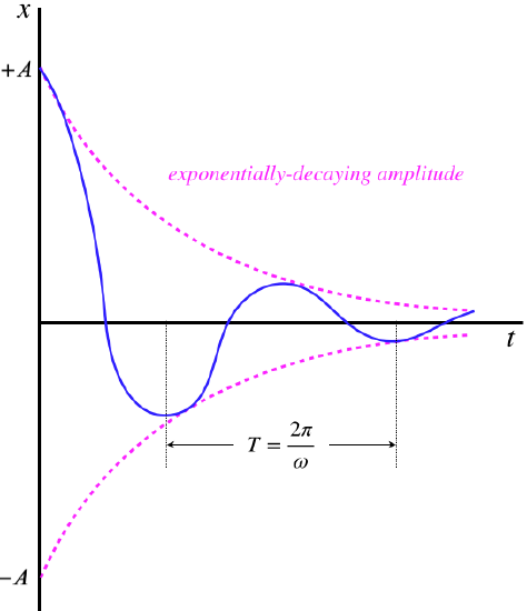
[Note: This graph starts at \(t=0\) with \(x=+A\) in order to simplify the picture of the exponential envelope. This means we have started the motion at rest at its maximum separation, which corresponds to a phase angle of \(\phi = \frac{\pi}{2}\).]
The effect on the energy of the system is obvious – the non-conservative drag force converts mechanical energy in the system into thermal energy, which is manifested as ever-decreasing amplitude (recall the simple relationship total energy has to amplitude, shown in Equation 8.1.12). Notice that if we gradually start increasing the value of \(\beta\), the period \(T\) gets longer, stretching out the spacing of the bumps on the graph (and moving the point where the graph first crosses the \(t\)-axis to the right), while at the same time making the exponential decay (the pink curve) steeper. It should not be surprising therefore what we find in the next case...
Case 2: \(\beta = 2\sqrt{km}\)
In this case, the sinusoidal behavior goes away. One way to see this is to note that this condition causes \(\omega\) to vanish, making the period infinite, thereby making it so that the system never completes an oscillation. This kind of motion is called critically-damped. The easiest way to get a handle on this is to simply plug the condition into the solution, Equation 8.3.4:
\[x\left(t\right) = \left[A\sin\phi\right]e^{-\sqrt\frac{k}{m} t}\]
We see that the oscillatory motion is gone (the sine function just includes the phase constant, so there is no time dependence in the sine function. In fact, if we start the motion at rest at the maximum spring stretch (\(\phi = \frac{\pi}{2}\), the value of \(x\left(t\right)\) never even goes negative – it just exponentially decays, and is simply one of the dashed pink graphs shown in Figure 8.3.1.
Case 3: \(\beta > 2\sqrt{km}\)
This is strange case is called overdamped. The value under the radical is now negative, which makes the angular frequency imaginary. Dealing with the complex numbers is a bit cumbersome, but fortunately we don't have to do this. We can simply go back to the original differential equation armed with the knowledge about \(\beta\) and obtain a new solution from scratch. Again, we are not in a position to delve into the details of solving differential equations, but this case also results in no oscillations, and exponential decay of the displacement toward the equilibrium point without ever crossing it. As one might expect, with a stronger force opposing the motion than the critically-damped case, the system heads toward the equilibrium point more slowly than that case.
Resonance
If we can take energy out of the system with a damping force that acts in opposition to the motion, it makes sense that we can also add energy into the system by introducing a force in the direction of motion. While a damping force by something like drag through a fluid works "automatically," adding energy to the system requires some coordination in the application of the force. For example, if the force can only act in the \(+x\) direction, the force can only be applied periodically – exerting it all the time would have it acting in the direction opposite to its motion half the time.
Generally when we talk about one of these energy-adding forces, we assume they are periodic (we call this a periodic driving force). The simplest such force is sinusoidal:
\[F\left(t\right) = F_o\sin\omega_dt\]
The quantity \(F_o\) is the maximum force applied, and \(\omega_d\) is the driving frequency. If we add this to the equation for Newton's second law (including damping), we get:
\[F_{net} = ma \;\;\;\Rightarrow\;\;\; -kx-\beta \dfrac{dx}{dt}+ F_o\sin\omega_dt = m\dfrac{d^2x}{dt^2}\]
These differential equations just keep getting uglier! We won't go into the solution for this one, but a look at the physical effects from a perspective of energy is enlightening.
The first thing we note is that this force, over time, adds energy to the system, which means that while the damping force takes energy away, the total energy doesn't decay all the way to zero. This means that an amplitude of oscillation doesn't dissipate away. Second, it seems clear that the more time that the force spends pushing in the correct direction, the more energy it can add to the system. It will maximize its pushing in the correct direction when it is completely synchronized with the natural or resonant frequency \(\omega_o \equiv \sqrt{\dfrac{k}{m}}\) of the system, which is the frequency at which it would oscillate without damping. To see this, we'll take a peek at the result of solving the differential equation. This solution gives the following expression for the amplitude resulting from forced, damped oscillatory motion:
\[A=\dfrac{F_o}{\sqrt{m^2\left(\omega_d^2-\omega_o^2\right)^2+\beta^2\omega_d^2}}\]
We can see from this expression that the closer the driving frequency \(\omega_d\) is to the natural frequency \(\omega_o\), the larger the amplitude is. Given that the amplitude is a proxy for the energy in the system, this means that more energy is added to the system by a driving force whose frequency is well-tuned to the natural frequency of the system. This phenomenon is called resonance.