
2.2: The Ellipse
- Page ID
- 6793

An ellipse is a figure that can be drawn by sticking two pins in a sheet of paper, tying a length of string to the pins, stretching the string taut with a pencil, and drawing the figure that results. During this process, the sum of the two distances from pencil to one pin and from pencil to the other pin remains constant and equal to the length of the string. This method of drawing an ellipse provides us with a formal definition, which we shall adopt in this chapter, of an ellipse, namely:
An ellipse is the locus of a point that moves such that the sum of its distances from two fixed points called the foci is constant (see figure II.6).
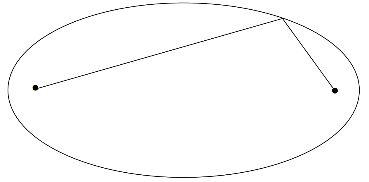
\(\text{FIGURE II.6}\)
We shall call the sum of these two distances (i.e the length of the string) \(2a\). The ratio of the distance between the foci to length of the string is called the eccentricity \(e\) of the ellipse, so that the distance between the foci is \(2ae\), and \(e\) is a number between 0 and 1.
The longest axis of the ellipse is its major axis, and a little bit of thought will show that its length is equal to the length of the string; that is, \(2a\). The shortest axis is the minor axis, and its length is usually denoted by \(2b\). The eccentricity is related to the ratio \(b/a\) in a manner that we shall shortly discuss.
The ratio
\[η = (a − b)/a\]
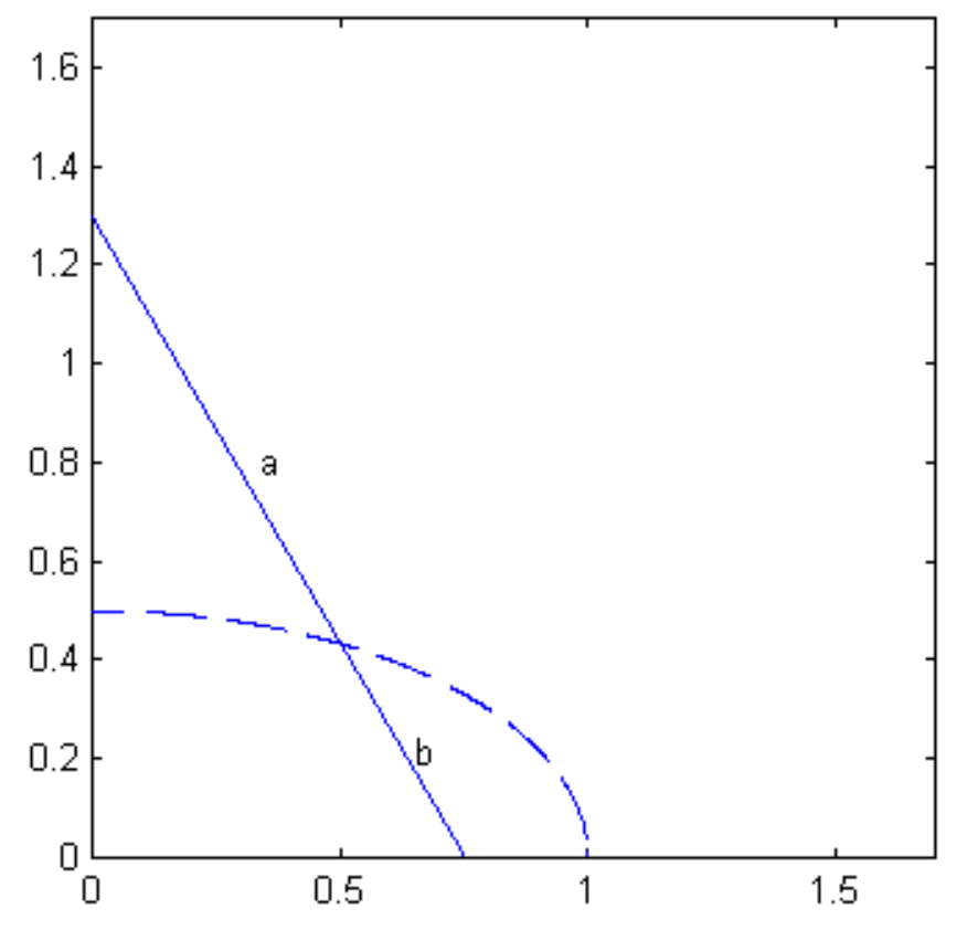
is called the ellipticity if the ellipse. It is merely an alternative measure of the noncircularity. It is related to the eccentricity, and we shall obtain that relation shortly, too. Until then, Figure \(\text{II.7}\) shows pictorially the relation between the two.
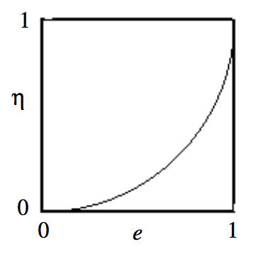
\(\text{FIGURE II.7}\)
We shall use our definition of an ellipse to obtain its Equation in rectangular coordinates. We shall place the two foci on the \(x\)-axis at coordinates (−\(ae\), 0) and (\(ae\), 0) (see figure II.8).
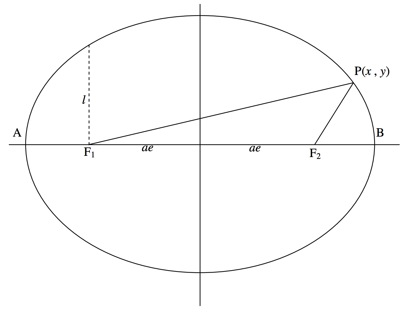
\(\text{FIGURE II.8}\)
The definition requires that \(\textbf{PF}_1 + \textbf{PF}_2 = 2a\). That is:
\[\left[ (x + ae)^2 + y^2 \right]^{\frac{1}{2}} + \left[ (x-ae)^2 + y^2 \right]^{\frac{1}{2}} = 2a, \label{2.3.1} \tag{2.3.1}\]
and this is the Equation to the ellipse. The reader should be able, after a little bit of slightly awkward algebra, to show that this can be written more conveniently as
\[\frac{x^2}{a^2} + \frac{y^2}{a^2(1-e^2)} = 1 . \label{2.3.2} \tag{2.3.2}\]
By putting \(x = 0\), it is seen that the ellipse intersects the \(y\)-axis at \(\pm a \sqrt{1-e^2}\) and therefore that \(a \sqrt{1-e^2}\) is equal to the semi minor axis \(b\). Thus we have the familiar Equation to the ellipse
\[\frac{x^2}{a^2} + \frac{y^2}{b^2} = 1 \label{2.3.3} \tag{2.3.3}\]
as well as the important relation between \(a\), \(b\) and \(e\):
\[b^2 = a^2 (1-e^2) \label{2.3.4} \tag{2.3.4}\]
The reader can also now derive the relation between ellipticity \(η\) and eccentricity \(e\):
\[η = 1 - \sqrt{(1-e^2)}. \label{2.3.5} \tag{2.3.5}\]
This can also be written
\[e^2 = \sqrt{η(2-η)} \label{2.3.6} \tag{2.3.6}\]
or \[e^2 + (η -1)^2 = 1. \label{2.3.7} \tag{2.3.7}\]
This shows, incidentally, that the graph of \(η\) versus \(e\), which we have drawn in figure \(\text{II.7}\), is part of a circle of radius 1 centred at \(e = 0, \ η = 1\).
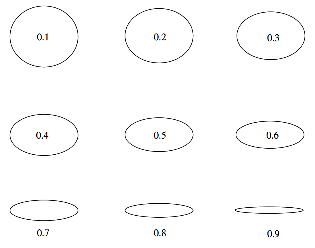
In figures \(\text{II.9}\) I have drawn ellipses of eccentricities 0.1 to 0.9 in steps of 0.1, and in figure \(\text{II.10}\) I have drawn ellipses of ellipticities 0.1 to 0.9 in steps of 0.1. You may find that ellipticity gives you a better idea than eccentricity of the noncircularity of an ellipse. For an exercise, you should draw in the positions of the foci of each of these ellipses, and decide whether eccentricity or ellipticity gives you a better idea of the "ex-centricity" of the foci. Note that the eccentricities of the orbits of Mars and Mercury are, respectively, about 0.1 and 0.2 (these are the most eccentric of the planetary orbits except for comet-like Pluto), and it is difficult for the eye to see that they depart at all from circles - although, when the foci are drawn, it is obvious that the foci are "ex-centric".
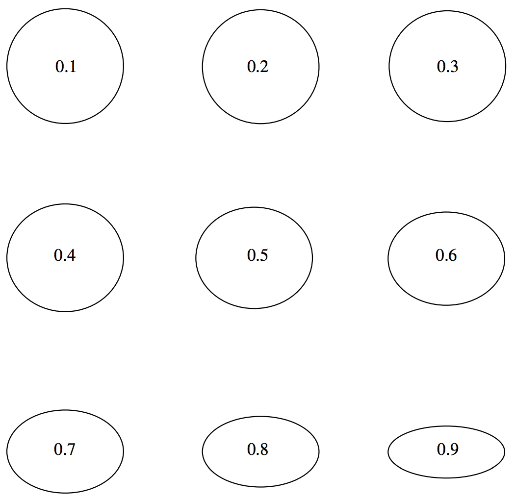
\(\text{FIGURE II.9}\): The number inside each ellipse is its eccentricity.
\(\text{FIGURE II.10}\): The figure inside or below each ellipse is its ellipticity.
In the theory of planetary orbits, the Sun will be at one focus. Let us suppose it to be at \(\text{F}_2\) (see figure \(\text{II.8}\)). In that case the distance \(\text{F}_2 \ \text{B}\) is the perihelion distance \(q\), and is equal to
\[q = a(1-e). \label{2.3.8} \tag{2.3.8}\]
The distance \(\text{F}_2 \ \text{A}\) is the aphelion distance Q (pronounced ap-helion by some and affelion by others − and both have defensible positions), and it is equal to
\[Q = a(1 + e). \label{2.3.9} \tag{2.3.9}\]
A line parallel to the minor axis and passing through a focus is called a latus rectum (plural: latera recta). The length of a semi latus rectum is commonly denoted by \(l \)(sometimes by \(p\)). Its length is obtained by putting \(x = ae\) in the Equation to the ellipse, and it will be readily found that
\[l = a(1-e^2). \label{2.3.10} \tag{2.3.10}\]
The length of the semi latus rectum is an important quantity in orbit theory. It will be found, for example, that the energy of a planet is closely related to the semi major axis \(a\) of its orbit, while its angular momentum is closely related to the semi latus rectum.
The circle whose diameter is the major axis of the ellipse is called the eccentric circle or, preferably, the auxiliary circle (figure \(\text{II.11}\)). Its Equation is
\[x^2 + y^2 = a^2 . \label{2.3.11} \tag{2.3.11}\]
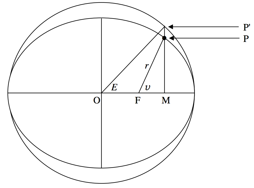
\(\text{FIGURE II.11}\)
In orbit theory the angle \(v\) (denoted by \(f\) by some authors) is called the true anomaly of a planet in its orbit. The angle \(E\) is called the eccentric anomaly, and it is important to find a relation between them.
We first note that, if the eccentric anomaly is \(E\), the abscissas of \(\text{P}^\prime\) and of \(\text{P}\) are each \(a \cos E\). The ordinate of \(\text{P}^\prime\) is \(a \sin E\). By putting \(x = a \cos E\) in the Equation to the ellipse, we immediately find that the ordinate of \(\text{P}\) is \(b \sin E\). Several deductions follow. One is that any point whose abscissa and ordinate are of the form
\[x = a \cos E , \quad y = b \sin E \label{2.3.12} \tag{2.3.12}\]
is on an ellipse of semi major axis \(a\) and semi minor axis \(b\). These two Equations can be regarded as parametric Equations to the ellipse. They can be used to describe an ellipse just as readily as
\[\frac{x^2}{a^2} + \frac{y^2}{b^2} = 1 \label{2.3.13} \tag{2.3.13}\]
and indeed this Equation is the \(E\)-eliminant of the parametric Equations.
The ratio \(\text{PM}/\text{P}^\prime \text{M}\) for any line perpendicular to the major axis is \(b/a\). Consequently the area of the ellipse is \(b/a\) times the area of the auxiliary circle; and since the area of the auxiliary circle is \(\pi a^2\), it follows that the area of the ellipse is \(\pi ab\).
In figure \(\text{II.11}\), the distance \(r\) is called the radius vector (plural radii vectores), and from the theorem of Pythagoras its length is given by
\[r^2 = b^2 \sin^2 E + a^2 (\cos E - e)^2 . \label{2.3.14} \tag{2.3.14}\]
On substituting \(1 − \cos^2 E\) for \(\sin^2 E\) and \(a^2 (1 - e^2 )\) for \(b^2\), we soon find that
\[r = a (1 - e \cos E ) \label{2.3.15} \tag{2.3.15}\]
It then follows immediately that the desired relation between \(v\) and \(E\) is
\[\cos v = \frac{\cos E - e}{1 - e \cos E} . \label{2.3.16} \tag{2.3.16}\]
From trigonometric identities, this can also be written
\[\sin v = \frac{\sqrt{1-e^2} \sin E}{1-e \cos E} \tag{2.3.17a} \label{2.3.17a}\]
or \[\tan v = \frac{\sqrt{1-e^2} \sin E}{\cos E - e} \label{2.3.17b} \tag{2.3.17b}\]
or \[ \tan \frac{1}{2} v = \sqrt{\frac{1+e}{1-e}} \tan \frac{1}{2} E . \label{2.3.17c} \tag{2.3.17c}\]
The inverse formulas may also be useful:
\[\cos E = \frac{e+\cos v}{1+e \cos v} \label{2.3.17d} \tag{2.3.17d}\]
\[\sin E = \frac{\sin v \sqrt{1-e^2}}{1 + e ~ \cos v} \label{2.3.17e} \tag{2.3.17e}\]
\[\tan E = \frac{\sin v \sqrt{1-e^2}}{e+ \cos v} \label{2.3.17f} \tag{2.3.17f}\]
\[\tan \frac{1}{2} E = \sqrt{\frac{1-e}{1+e}} \tan \frac{1}{2} v . \label{2.3.17g} \tag{2.3.17g}\]
There are a number of miscellaneous geometric properties of an ellipse, some, but not necessarily all, of which may prove to be of use in orbital calculations. We describe some of them in what follows.
Tangents to an Ellipse
Find where the straight line \(y = mx + c\) intersects the ellipse
\[\frac{x^2}{a^2} + \frac{y^2}{b^2} = 1 . \label{2.3.18} \tag{2.3.18}\]
The answer to this question is to be found by substituting \(mx + c\) for \(y\) in the Equation to the ellipse. After some rearrangement, a quadratic Equation in \(x\) results:
\[\left(a^2 m^2 + b^2 \right) x^2 + 2a^2 cmx + a^2 \left( c^2 - b^2 \right) = 0 . \label{2.3.19} \tag{2.3.19}\]
If this Equation has two real roots, the roots are the \(x\)-coordinates of the two points where the line intersects the ellipse. If it has no real roots, the line misses the ellipse. If it has two coincident real roots, the line is tangent to the ellipse. The condition for this is found by setting the discriminant of the quadratic Equation to zero, from which it is found that
\[c^2 = a^2 m^2 + b^2 . \label{2.3.20} \tag{2.3.20}\]
Thus a straight line of the form
\[y = mx \pm \sqrt{a^2 m^2 + b^2} \label{2.3.21} \tag{2.3.21}\]
is tangent to the ellipse.
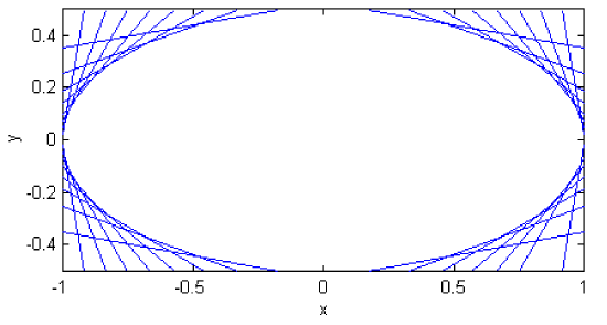
Figure \(\text{II.12}\) shows several such lines, for \(a = 2b\) and slopes (\(\tan^{-1} \ m)\) of \(0^\circ\) to \(180^\circ\) in steps of \(10^\circ\)
\(\text{FIGURE II.12}\)
Director Circle
The Equation we have just derived for a tangent to the ellipse can be rearranged to read
\[m^2 \left( a^2 - x^2 \right) + 2mx + b^2 - y^2 = 0. \label{2.3.22} \tag{2.3.22} \]
Now the product of the slopes of two lines that are at right angles to each other is \(−1\) (Equation 2.2.17). Therefore, if we replace \(m\) in the above Equation by \(−1/m\) we shall obtain another tangent to the ellipse, at right angles to the first one. The Equation to this second tangent becomes (after multiplication throughout by \(m\) )
\[m^2 \left( b^2 - y^2 \right) - 2mx + a^2 - x^2 = 0. \label{2.3.23} \tag{2.3.23}\]
If we eliminate \(m\) from these two Equations, we shall obtain an Equation in \(x\) and \(y\) that describes the point where the two perpendicular tangents meet; that is, the Equation that will describe a curve that is the locus of the point of intersection of two perpendicular tangents. It turns out that this curve is a circle of radius \(\sqrt{a^2 + b^2}\), and it is called the director circle.
It is easier than it might first appear to eliminate \(m\) from the Equations. We merely have to add the Equations \(\ref{2.3.22}\) and \(\ref{2.3.23}\):
\[m^2 \left( a^2 + b^2 - x^2 - y^2 \right) + a^2 + b^2 - x^2 - y^2 = 0 . \label{2.3.24} \tag{2.3.24}\]
For real \(m\), this can only be if
\[x^2 + y^2 = a^2 + b^2 , \label{2.3.25} \tag{2.3.25}\]
which is the required locus of the director circle of radius \(\sqrt{a^2 + b^2}\). It is illustrated in figure \(\text{II.13}\).
We shall now derive an Equation to the line that is tangent to the ellipse at the point \((x_1 , \ y_1 )\).
Let \((x_1 , \ y_1 ) = (a \cos E_1 , b \sin E_1 )\) and \((x_2 , \ y_2 ) = (a \cos E_2 , b \sin E_2 )\) be two points on the ellipse.
The line joining these two points is
\[\frac{y-b\sin E_1}{x-a \cos E_1} = \frac{b ( \sin E_2 - \sin E_1 )}{a(\cos E_2 - \cos E_1 )} = \frac{2b \cos \frac{1}{2}(E_2 + E_1) \sin \frac{1}{2}(E_2 - E_1)}{-2a \sin \frac{1}{2} (E_2 + E_1) \sin \frac{1}{2}(E_2 - E_1)} = -\frac{b \cos \frac{1}{2} (E_2 + E_1)}{a \sin \frac{1}{2} (E_2 + E_1)}. \label{2.3.26} \tag{2.3.26}\]
\(\text{FIGURE II.13}\)
Now let \(E_2\) approach \(E_1\), eventually coinciding with it. The resulting Equation
\[\frac{y-b\sin E}{x - a \cos E} = - \frac{b \cos E}{a \sin E} , \label{2.3.27} \tag{2.3.27}\]
in which we no longer distinguish between \(E_1\) and \(E_2\), is the Equation of the straight line that is tangent to the ellipse at \((a \cos E \ , b \sin E )\). This can be written
\[\frac{x \cos E}{a} + \frac{y \sin E}{b} = 1 \label{2.3.28} \tag{2.3.28}\]
or, in terms of \((x_1 , \ y_1 )\),
\[\frac{x_1 x}{a^2} + \frac{y_1 y}{b^2} = 1, \label{2.3.29} \tag{2.3.29}\]
which is the tangent to the ellipse at \((x_1 , \ y_1 )\).
An interesting property of a tangent to an ellipse, the proof of which I leave to the reader, is that \(\text{F}_1 \text{P}\) and \(\text{F}_2 \text{P}\) make equal angles with the tangent at \(\text{P}\). If the inside of the ellipse were a reflecting mirror and a point source of light were to be placed at \(\text{F}_1\), it would be imaged at \(\text{F}_2\). (Have a look at figure \(\text{II.6}\) or \(\text{II.8}\).) This has had an interesting medical application. A patient has a kidney stone. The patient is asked to lie in an elliptical bath, with the kidney stone at \(\text{F}_2\). A small explosion is detonated at \(\text{F}_1\); the explosive sound wave emanating from \(\text{F}_1\) is focused as an implosion at \(\text{F}_2\) and the kidney stone at \(\text{F}_2\) is shattered. Don't try this at home.
Directrices
The two lines \(x = \pm a / e\) are called the directrices (singular directrix) of the ellipse (figure \(\text{II.14}\)).
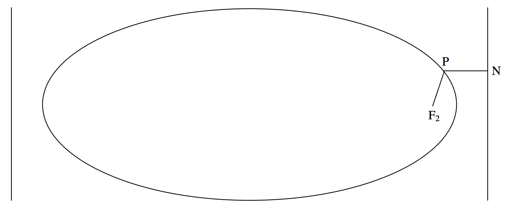
\(\text{FIGURE II.14}\)
The ellipse has the property that, for any point \(\text{P}\) on the ellipse, the ratio of the distance \(\text{PF}_2\) to a focus to the distance \(\text{PN}\) to a directrix is constant and is equal to the eccentricity of the ellipse. Indeed, this property is sometimes used as the definition of an ellipse, and all the Equations and properties that we have so far derived can be deduced from such a definition. We, however, adopted a different definition, and the focus-directrix property must be derived. This is straightforward, for, (recalling that the abcissa of \(\text{F}_2\) is \(ae\)) we see from figure \(\text{II.14}\) that the square of the desired ratio is
\[\frac{(x - a e)^2 + y^2}{(a/e-x)^2}. \label{2.3.30} \tag{2.3.30}\]
On substitution of
\[b^2 \left( 1 - \left( \frac{x}{a} \right)^2 \right) = a^2 \left( 1 - e^2 \right) \left( 1 - \left( \frac{x}{a} \right)^2 \right) = \left( 1 - e^2 \right) \left( a^2 - x^2 \right) \label{2.3.31} \tag{2.3.31}\]
for \(y^2\), the above expression is seen to reduce to \(e^2\).
Another interesting property of the focus and directrix, although a property probably with not much application to orbit theory, is that if the tangent to an ellipse at a point \(\text{P}\) intersects the directrix at \(\text{Q}\), then \(\text{P}\) and \(\text{Q}\) subtend a right angle at the focus. (See figure \(\text{II.15}\)).
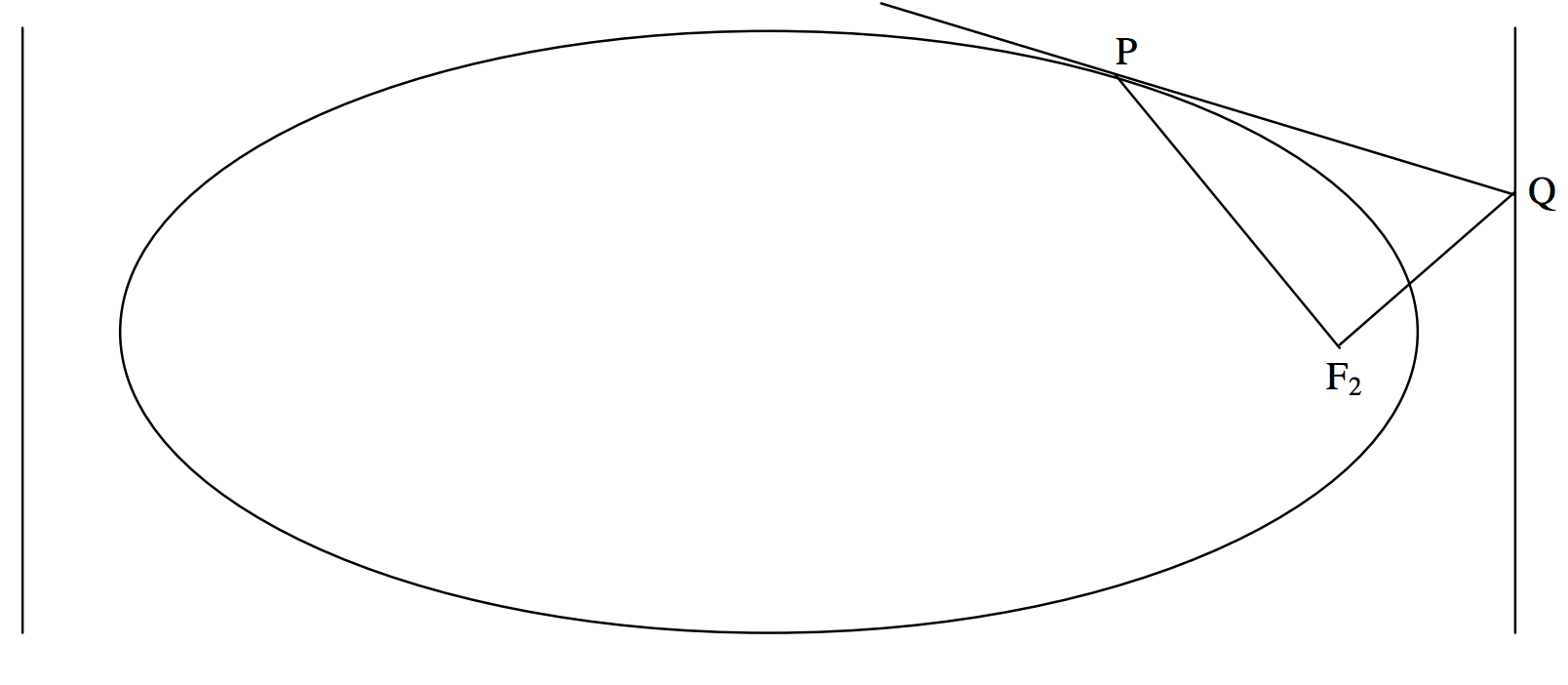
\(\text{FIGURE II.15}\)
Thus the tangent at \(\text{P} = (x_1 , \ y_1 )\) is
\[\frac{x_1 x}{a^2} + \frac{y_1 y }{b^2} = 1 \label{2.3.32} \tag{2.3.32}\]
and it is straightforward to show that it intersects the directrix \(x = a/e\) at the point
\[\left( \frac{a}{e} , \frac{b^2}{y_1} \left( 1 - \frac{x_1}{ae} \right) \right) . \]
The coordinates of the focus \(\text{F}_2\) are \((ae, 0)\). The slope of the line \(\text{PF}_2\) is \((x_1 - ae )/y_1\) and the slope of the line \(\text{QF}_2\) is
\[\frac{\frac{b^2}{y_1} \left( 1 - \frac{x_1}{ae} \right)}{\frac{a}{e} - ae}. \]
It is easy to show that the product of these two slopes is \(−1\), and hence that \(\text{PF}_2\) and \(\text{QF}_2\) are at right angles.
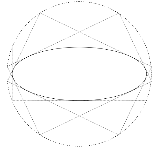
Conjugate Diameters
The left hand of figure \(\text{II.16}\) shows a circle and two perpendicular diameters. The right hand figure shows what the circle would look like when viewed at some oblique angle. The circle has become an ellipse, and the diameters are no longer perpendicular. The diameters are called conjugate diameters of the ellipse. One is conjugate to the other, and the other is conjugate to the one. They have the property - or the definition - that each bisects all chords parallel to the other, because this property of bisection, which is obviously held by the perpendicular diameters of the circle, is unaltered in projection.
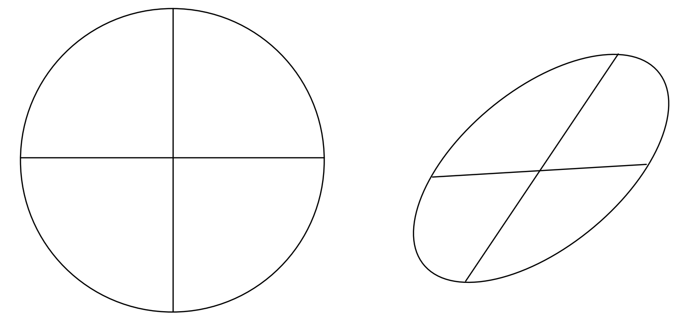
\(\text{FIGURE II.16}\)
It is easy to draw two conjugate diameters of an ellipse of eccentricity \(e\) either by making use of this last-mentioned property or by noting that that the product of the slopes of two conjugate diameters is \(e^2 − 1\). The proof of this is left for the enjoyment of the reader.
A Ladder Problem.
No book on elementary applied mathematics is complete without a ladder problem. A ladder of length \(a + b\) leans against a smooth vertical wall and a smooth horizontal floor. A particular rung is at a distance \(a\) from the top of the ladder and \(b\) from the bottom of the ladder. Show that, when the ladder slips, the rung describes an ellipse. (This result will suggest another way of drawing an ellipse.) See figure \(\text{II.17}\).
\(\text{FIGURE II.17}\)
If you have not done this problem after one minute, here is a hint. Let the angle that the ladder makes with the floor at any time be \(E\). That is the end of the hint.
The reader may be aware that some of the geometrical properties that we have discussed in the last few paragraphs are more of recreational interest and may not have much direct application in the theory of orbits. In the next subsection we return to properties and Equations that are very relevant to orbital theory - perhaps the most important of all for the orbit computer to understand.
Polar Equation to the Ellipse
We shall obtain the Equation in polar coordinates to an ellipse whose focus is the pole of the polar coordinates and whose major axis is the initial line \((\theta = 0^\circ )\) of the polar coordinates. In figure \(\text{II.18}\) we have indicated the angle \(\theta\) of polar coordinates, and it may occur to the reader that we have previously used the symbol \(v\) for this angle and called it the true anomaly. Indeed at present, \(v\) and \(\theta\) are identical, but a little later we shall distinguish between them.
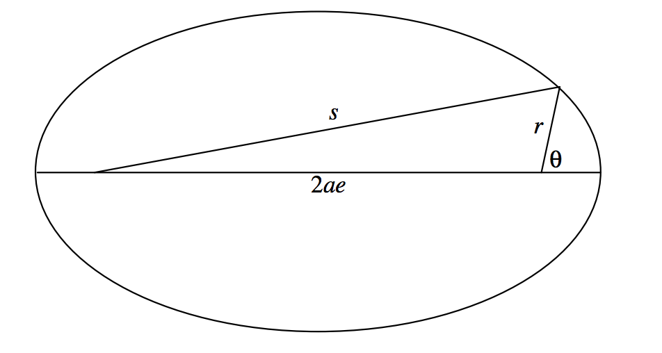
\(\text{FIGURE II.18}\)
From our definition of the ellipse, \(s = 2a − r\), and so
\[s^2 = 4a^2 - 4ar + r^2 . \label{2.3.33} \tag{2.3.33}\]
From the cosine formula for a plane triangle,
\[s^2 = 4a^2 e^2 + r^2 + 4aer \cos \theta . \label{2.3.34} \tag{2.3.34}\]
On equating these expressions we soon obtain
\[a \left( 1 - e^2 \right) = r \left( 1 + e \cos \theta \right) . \label{2.3.35} \tag{2.3.35} \]
The left hand side is equal to the semi latus rectum \(l\), and so we arrive at the polar Equation to the ellipse, focus as pole, major axis as initial line:
\[r = \frac{1}{1+e \cos \theta}. \label{2.3.36} \tag{2.3.36}\]
If the major axis is inclined at an angle \(ω\) to the initial line (figure \(\text{II.19}\) ), the Equation becomes
\[r = \frac{l}{1 + e \cos (\theta - ω)} = \frac{l}{1+ e \cos v}. \label{2.3.37} \tag{2.3.37}\]
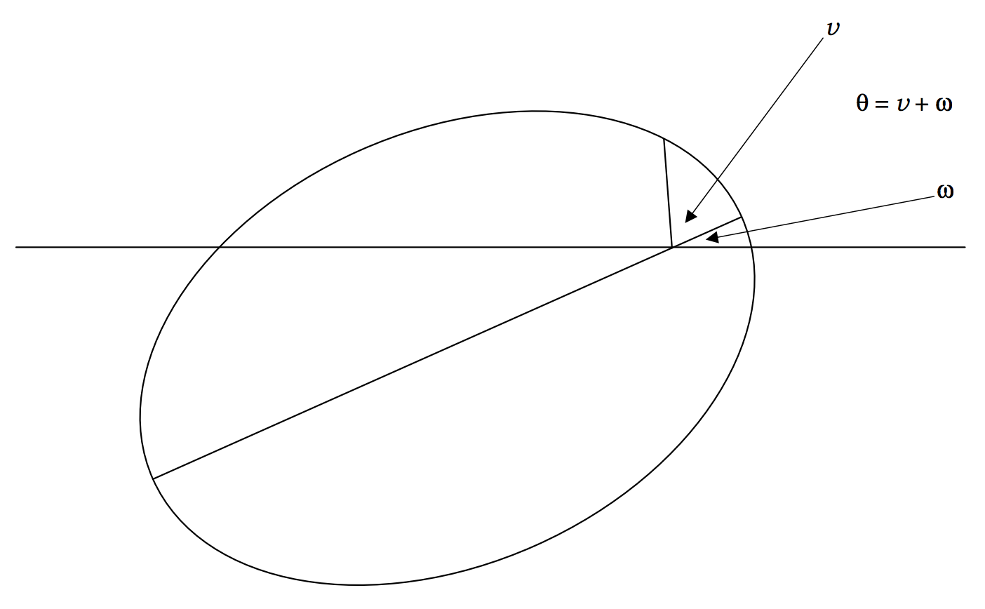
\(\text{FIGURE II.19}\)
The distinction between \(θ\) and \(v\) is now evident. \(θ\) is the angle of polar coordinates, \(ω\) is the angle between the major axis and the initial line (\(ω\) will be referred to in orbital theory as the "argument of perihelion"), and \(v\), the true anomaly, is the angle between the radius vector and the initial line.