9.6: LS-coupling

The expression 9.5.2 gives the transition moment for a component, and its square is the strength of the component. For the strength of a line, one merely adds the strengths of the components. In general it is very hard to calculate the transition moment accurately in absolute units.

In LS-coupling, the strength of a line can be written as the product of three factors:

\[S = \mathcal{S} (\text{M}) \text{S} (\text{L}) \sigma^2 . \label{9.6.1}\]

Here \(\sigma^2\) is the strength of the transition array, and is given by

\[\sigma^2 = \frac{e^2}{4l^2 -1} \left( \int_0^\infty r^3 R_i R_f dr \right)^2 . \label{9.6.2}\]

Here \(l\) is the larger of the two azimuthal quantum numbers involved in the transition. \(R_i\) and \(R_f\) are the radial parts of the initial and final wavefunctions (each of which has dimension \(\text{L}^{-3/2}\)). The reader should verify that the expression \(\ref{9.6.2}\) has dimensions of the square of electric dipole moment. In general \(\sigma^2\) (which is the only dimensioned term on the right hand side of Equation \(\ref{9.6.1}\)) is difficult to calculate, and it determines the absolute scale of the line strengths. Unless the strength of the transition array can be determined (in \(\text{C}^2 \text{ m}^2\) or equivalently in atomic units of \(a_0^2 e^2\)), absolute values of line strengths will remain unknown. However, for \(LS\)-coupling, there exist explicit algebraic expressions for \(\mathcal{S}(\text{M})\), the relative strengths of the multiplets within the array, and for \(\mathcal{S}(\text{L})\), the relative strengths of the lines within a multiplet. In this section I give the explicit formulas for the relative strengths of the lines within a multiplet.

In \(LS\)-coupling there are two types of multiplet – those in which \(L\) changes by 1, and those in which \(L\) does not change. I deal first with multiplets in which \(L\) changes by 1. In the following formulas, \(L\) is the larger of the two orbital angular momentum quantum numbers involved. For multiplets connecting two \(LS\)-coupled terms, \(S\) is the same in each term. The selection rule for \(J\) is \(\Delta J = 0, \pm 1\). The lines in which \(J\) changes in the same way as \(L\) (i.e. if \(L\) increases by 1, \(J\) also increases by 1) are the strongest lines in the multiplet, and are called the main lines or the principal lines. The lines in which \(J\) does not change are weaker (“satellite” lines), and the lines in which the change in \(J\) is in the opposite sense to the change in \(L\) are the weakest (“second satellites”). Some of the following formulas include the factor \((−1)^2\). This is included so that the transition moment (the square root of the line strength) can be recovered if need be.

\(\underline{\text{Multiplet } L \text{ to } L - 1}.\)

Main lines, \(J\) to \(J − 1\):

\[\mathcal{S}(\text{L}) = \frac{(J+L-S-1) (J+L-S) (J+L+S+1)(J+L+S)}{4JL(4L^2-1)(2S+1)} \label{9.6.3}\]

First satellites (weaker lines), no change in \(J\):

\[\mathcal{S}(\text{L}) = \frac{(2J+1) (J+L-S)(J-L+S+1)(J+L+S+1)(-J+L+S)}{4J(J+1)L(4L^2-1)(2S+1)} \label{9.6.4}\]

Second satellites (weakest lines), \(J\) to \(J + 1\):

\[\mathcal{S} (\text{L}) = \frac{(-1)^2 (J-L+S+1)(-J+L+S)(J-L+S+2)(-J+L+S-1)}{4(J+1)L(4L^2-1)(2S+1)} \label{9.6.5}\]

Example \(\PageIndex{1}\)

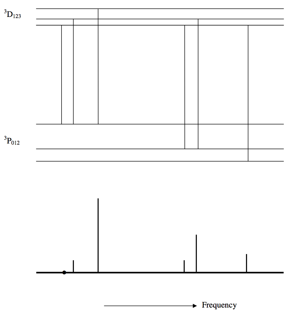
The multiplet \(^3 \text{P} − \ ^3\text{D}\). Here, we have \(S = 1\), and \(L = 2\).

There are six lines. In what follows I list them, together with the \(J\) value to be substituted in the formulas, and the value of \(\mathcal{S}(\text{L})\).

\begin{array}{c l c c c c c}
^3 \text{P}_0 - \ ^3\text{D}_1 & \text{Main} & J=1 & \mathcal{S}(\text{L}) & = & 1/9 & = & 0.11111 \\
\\
^3 \text{P}_1 - \ ^3\text{D}_2 & \text{Main} & J=2 & \mathcal{S}(\text{L}) & = & 1/4 & = & 0.25000 \\
^3 \text{P}_1 - \ ^3\text{D}_1 & \text{First satellite} & J=1 & \mathcal{S}(\text{L}) & = & 1/12 & = & 0.08333 \\
\\
^3 \text{P}_2 - \ ^3\text{D}_3 & \text{Main} & J=3 & \mathcal{S}(\text{L}) & = & 7/15 & = & 0.46667 \\
^3 \text{P}_2 - \ ^3\text{D}_2 & \text{First satellite} & J=2 & \mathcal{S}(\text{L}) & = & 1/12 & = & 0.08333 \\
^3 \text{P}_2 - \ ^3\text{D}_1 & \text{Second satellite} & J=1 & \mathcal{S}(\text{L}) & = & 1/180 & = & 0.00556 \\
\nonumber
\end{array}

The transitions and the positions and intensities of the lines are illustrated in figure IX.2.

It was mentioned in Chapter 7 that one of the tests for \(LS\)-coupling was Hund’s interval rule, which governs the spacings of the levels within a term, and hence the wavelength spacings of the lines within a multiplet. Another test is that the relative intensities of the lines within a multiplet follow the line strength formulas for \(LS\)-coupling. The characteristic spacings and intensities form a “fingerprint” by which \(LS\)-coupling can be recognized. It is seen in the present case \((^3 \text{P} − \ ^3\text{D})\) that there are three main lines, the strongest of which has two satellites, and the second strongest has one satellite.

\(\text{FIGURE IX.2}\)

The second type of multiplet is the symmetric multiplet, in which there is no change in \(L\) − for example, \(^3 \text{P} − \ ^3 \text{P}\). The strongest lines (main lines) are those in which there is no change in \(J\).

The formulas for the relative line strengths within a symmetric multiplet are:

Main lines, no change in J:

\[\mathcal{S}(\text{L}) = \frac{(2J+1)[J(J+1)+L(L+1)-S(S+1)]^2}{4J(J+1)L(L+1)(2L+1)(2S+1)} \label{9.6.6}\]

Satellite lines, \(J\) changes by \(\pm 1\); in the following formula, \(J\) is the larger of the two \(J\)-values:

\[\mathcal{S}(\text{L}) = \frac{(-1)^2 (J+L-S) (J-L+S) (J+L+S+1) (-J+L+S+1)}{4JL (L+1) (2L+1) (2S+1)} \label{9.6.7}\]

Example: \(^3 \text{D} - \ ^3\text{D}\):

\begin{array}{c l c c c c}
^3\text{D}_1 - \ ^3\text{D}_1 & \text{Main} & J=1 & \mathcal{S}(\text{L}) & = & 0.150000 \\
^3\text{D}_2 - \ ^3\text{D}_2 & \text{Main} & J=2 & \mathcal{S}(\text{L}) & = & 0.231481 \\
^3\text{D}_3 - \ ^3\text{D}_3 & \text{Main} & J=3 & \mathcal{S}(\text{L}) & = & 0.414815 \\
\\
^3\text{D}_2 - \ ^3\text{D}_3 & \text{Satellite} & J=3 & \mathcal{S}(\text{L}) & = & 0.051852 \\
^3\text{D}_1 - \ ^3\text{D}_2 & \text{Satellite} & J=2 & \mathcal{S}(\text{L}) & = & 0.050000 \\
^3\text{D}_3 - \ ^3\text{D}_2 & \text{Satellite} & J=3 & \mathcal{S}(\text{L}) & = & 0.051852 \\
^3\text{D}_2 - \ ^3\text{D}_1 & \text{Satellite} & J=2 & \mathcal{S}(\text{L}) & = & 0.050000 \\
\end{array}

I leave it to the reader to draw a figure analogous to figure \(\text{IX.2}\) for a symmetric multiplet. Remember that the spacings of the levels within a term are given by Equation 7.17.1, and you can use different coupling coefficients for the two terms. It should be easier for you to draw the levels and the transitions with pencil and ruler than for me to struggle to draw it with a computer.

Tabulations of these formulae are available in several places. Today, however, it is often quicker to calculate them with either a computer or hand calculator than to find one of the tabulations and figure out how to read it. (Interesting thought: It is quicker to draw an energy level diagram with pencil and paper than with a computer, but it is quicker to calculate line strengths by computer than to look them up in tables.)

The relative strengths of hyperfine components within a line can be calculated with the same formulae by substituting \(JIF\) for \(LSJ\), since \(JI\)-coupling is usual.