6.4: The Biot-Savart Law

Since we now know that a wire carrying an electric current is surrounded by a magnetic field, and we have also decided upon how we are going to define the intensity of a magnetic field, we want to ask if we can calculate the intensity of the magnetic field in the vicinity of various geometries of electrical conductor, such as a straight wire, or a plane coil, or a solenoid. When we were calculating the electric field in the vicinity of various geometries of charged bodies, we started from Coulomb’s Law, which told us what the field was at a given distance from a point charge. Is there something similar in electromagnetism which tells us how the magnetic field varies with distance from an electric current? Indeed there is, and it is called the Biot-Savart Law.

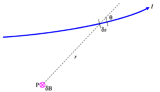
\(\text{FIGURE VI.3}\)

Figure VI.3 shows a portion of an electrical circuit carrying a current \(I\). The Biot-Savart Law tells us what the contribution \(\delta B\) is at a point \(\text{P}\) from an elemental portion of the electrical circuit of length \(\delta s\) at a distance \(r\) from \(\text{P}\), the angle between the current at \(\delta s\) and the radius vector from \(\text{P}\) to \(\delta s\) being \(q\). The Biot-Savart Law tells us that

\[\delta B ∝ \frac{I\delta s \sin \theta}{r^2}.\]

This law will enable us, by integrating it around various electrical circuits, to calculate the total magnetic field at any point in the vicinity of the circuit.

But – can I prove the Biot-Savart Law, or is it just a bald statement from nowhere? The answer is neither. I cannot prove it, but nor is it merely a bald statement from nowhere. First of all, it is a not unreasonable guess to suppose that the field is proportional to \(I\) and to \(\delta s\), and also inversely proportional to \(r^2\), since \(\delta s\), in the limit, approaches a point source. But you are still free to regard it, if you wish, as speculation, even if reasonable speculation. Physics is an experimental science, and to that extent you cannot “prove” anything in a mathematical sense; you can experiment and measure. The Biot-Savart law enables us to calculate what the magnetic field ought to be near a straight wire, near a plane circular current, inside a solenoid, and indeed near any geometry you can imagine. So far, after having used it to calculate the field near millions of conductors of a myriad shapes and sizes, the predicted field has always agreed with experimental measurement. Thus the Biot-Savart law is likely to be true – but you are perfectly correct in asserting that, no matter how many magnetic fields it has correctly predicted, there is always the chance that, some day, it will predict a field for some unusually-shaped circuit that disagrees with what is measured. All that is needed is one such example, and the law is disproved. You may, if you wish, try and discover, for a Ph.D. project, such a circuit; but I would not recommend that you spend your time on it!

There remains the question of what to write for the constant of proportionality. We are free to use any symbol we like, but, in modern notation, we symbol we use is \(\frac{\mu_0}{4\pi}\). Why the factor \(4\pi\)? The inclusion of \(4\pi\) gives us what is called a “rationalized” definition, and it is introduced for the same reasons that we introduced a similar factor in the constant of proportionality for Coulomb’s law, namely that it results in the appearance of \(4\pi\) in spherically-symmetric geometries, \(2\pi\) in cylindrically-symmetric geometries, and no \(\pi\) where the magnetic field is uniform. Not everyone uses this definition, and this will be discussed in a later chapter, but it is certainly the recommended one.

In any case, the Biot-Savart Law takes the form

\[\delta B = \frac{\mu_0}{4\pi}\frac{I\delta s \sin \theta}{r^2}.\label{6.4.2}\]

The constant \(\mu_0\) is called the permeability of free space, “free space” meaning a vacuum. The subscript allows for the possibility that if we do an experiment in a medium other than a vacuum, the permeability may be different, and we can then use a different subscript, or none at all. In practice the permeability of air is very little different from that of a vacuum, and hence I shall normally use the symbol \(\mu_0\) for experiments performed in air, unless we are discussing measurement of very high precision.

From Equation \ref{6.4.2}, we can see that the SI units of permeability are \(\text{T m A}^{-1}\) (tesla metres per amp). In a later chapter we shall come across another unit – the henry – for a quantity (inductance) that we have not yet described, and we shall see then that a more convenient unit for permeability is \(\text{H m}^{-1}\) (henrys per metre) – but we are getting ahead of ourselves.

What is the numerical value of \(\mu_0\)? I shall reveal that in the next chapter.

of permeability are \(\text{MLQ}^{-2}\). This means that you may, if you wish, express permeability in units of \(\text{kg m C}^{-2}\) – although you may get some queer looks if you do.

Thought for the Day.

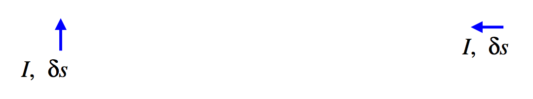
The sketch shows two current elements, each of length \(\delta s\), the current being the same in each but in different directions. Is the force on one element from the other equal but opposite to the force on the other from the one? If not, is there something wrong with Newton’s third law of motion? Discuss this over lunch.