
17.6: Linear Triatomic Molecule
- Page ID
- 7042

In Chapter 2, Section 2.9, we discussed a rigid triatomic molecule. Now we are going to discuss three masses held together by springs, of force constants \(k_1 \) and \(k_2\). We are going to allow it to vibrate, but not to rotate. Also, for the time being, I do not want the molecule to bend, so we’ll put it inside a drinking straw to that all the vibrations are linear. By the way, for real triatomic molecules, the force constants and rotational inertias are such that molecules vibrate much faster than they rotate. To see their vibrations you look in the near infra-red spectrum; to see their rotation, you have to go to the far infrared or the microwave spectrum.
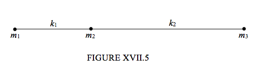
Suppose that the equilibrium separations of the atoms are \(a_1\) and \(a_2\). Suppose that at some instant of time, the x-coordinates (distances from the left hand edge of the page) of the three atoms are \(x_1, x_2 , x_3\). The extensions from the equilibrium distances are then \( q_1 = x_2 - x_1 - a_1, q_2 = x_3 - x_2 - a_2 \). We are now ready to start:
\[ T = \frac{1}{2}m_1\dot{x}^2_1 + \frac{1}{2}m_2\dot{x}^2_2 + \frac{1}{2}m_2\dot{x}^2_3, \label{17.6.1} \]
\[ V = \frac{1}{2}k_1q^2_1 + \frac{1}{2}k_2q^2_2. \label{17.6.2} \]
We need to express the kinetic energy in terms of the internal coordinate, and, just as for the diatomic molecule (Section 17.2), the relevant equations are
\[ \dot{q}_1 = \dot{x}_2- \dot{x}_1, \label{17.6.3} \]
\[ \dot{q}_2 = \dot{x}_3- \dot{x}_2, \label{17.6.4} \]
and
\[ 0 = m_1\dot{x}_1 + m_2\dot{x}_2 + m_3\dot{x}_3 . \label{17.6.5} \]
These can conveniently be written
\[ \begin{pmatrix}\dot{q}_1\\ \dot{q}_2 \\0\end{pmatrix} = \begin{pmatrix}-1 & 1 & 0 \\ 0 & -1 & 1\\ m_1 & m_2 & m_3\end{pmatrix}\begin{pmatrix}\dot{x}_1\\ \dot{x}_2 \\\dot{x}_3\end{pmatrix} \label{17.6.6} \]
By one dexterous flick of the fingers (!) we invert the matrix to obtain
\[ \begin{pmatrix}\dot{x}_1\\ \dot{x}_2 \\\dot{x}_3\end{pmatrix} = \begin{pmatrix}-\frac{m_2+m_3}{M} & -\frac{m_3}{M} & \frac{1}{M} \\ \frac{m_1}{M} & -\frac{m_3}{M} & \frac{1}{M}\\ \frac{m_1}{M} & \frac{m_1+m_2}{M} & \frac{1}{M}\end{pmatrix} \begin{pmatrix}\dot{q}_1\\ \dot{q}_2 \\0\end{pmatrix}, \label{17.6.7} \]
where \( M = m_1 + m_2 + m_3 \). On putting these into Equation \( \ref{17.6.1}\), we now have
\[ T = \frac{1}{2}(a\dot{q}^2_1 + 2h\dot{q}_1\dot{q}_2 + b\dot{q}^2_2) \label{17.6.8} \]
and
\[ V = \frac{1}{2}k_1q^2_1 + \frac{1}{2}k_2q^2_2 \label{17.6.2.} \]
where
\[ a = m_1(m_2+m_3)/M, \label{17.6.9} \]
\[ h = m_3m_1/M, \label{17.6.10} \]
\[ b = m_3(m_1+m_2)/M \label{17.6.11} \]
and for future reference,
\[ ab-h^2 = m_1m_2m_2 / M = m^2h. \label{17.6.12} \]
On application of Lagrange’s equation in turn to the two internal coordinates we obtain
\[ a\ddot{q}_1 + h\ddot{q}_2 + k_1q_1 = 0 \label{17.6.13} \]
and
\[ b\ddot{q}_2 + h\ddot{q}_2 + k_2q_2 = 0 \label{17.6.14} \]
Seek solutions of the form \( \ddot{q}_1 = - \omega^2 q_1 \) and \( \ddot{q}_2 = - \omega^2 q_2 \) and we obtain the following two expressions for the extension ratios:
\[ \frac{q_1}{q_2} = \frac{h \omega^2}{k_1-a \omega^2}= \frac{k_2 - b \omega^2}{h \omega ^2} . \label{17.6.15} \]
Equating them gives the equation for the normal mode frequencies:
\[ (ab - h^2)\omega^4 - (ak_2 + bk_1)\omega^2 + k_1k_2 = 0. \label{17.6.16} \]
For example, if \( k_1 = k_2 = l \) and \(m_1 = m_2 = m_3 = m \), we obtain, for the slow symmetric (“breathing”) mode, \(q_1/q_2 = +1 \) and \( \omega^2 = k/m \). For the fast asymmetric mode, \(q_1/q_2 = -1 \) and \(\omega^2 = 3k/m\).
Example.
Consider the linear OCS molecule whose atoms have masses 16, 12 and 32. Suppose that the angular frequencies of the normal modes, as determined from infrared spectroscopy, are 0.905 and 0.413. (I just made these numbers up, in unstated units, just for the purpose of illustrating the calculation. Without searching the literature, I can’t say what they are in the real OCS molecule.) Determine the force constants.
In Chapter 2 we considered a rigid triatomic molecule. We were given the moment of inertia, and we were asked to find the two internuclear distances. We couldn’t do this with just one moment of inertia, so we made an isotopic substitution (18O instead of 16O) to get a second equation, and so we could then solve for the two internuclear distances. This time, we are dealing with vibration, and we are going to use Equation \( \ref{17.6.16}\) to find the two force constants. This time, however, we are given two frequencies (of the normal modes), and so we have no need to make an isotopic substitution − we already have two equations.
Here are the necessary data.
16OCS
Fast \(\omega\) 0.905
Slow \(\omega\) 0.413
\(m_1 m_2 m_3 \) 16 12 32
\(M\) 60
\(a\) 11.73
\(h\) 8.53
\(b\) 14.93
\(ab − h^2\) 102.4
Use equation 17.6.16 for each of the frequencies, and you’ll get two equations, in \(k_1\) and \(k_2\). As in the rotational case, they are quadratic equations, but they are a bit easier to solve than in the rotational case. You’ll get two equations, each of the form of \( A - Bk_1 - Ck_2 + k_1k_2 = 0\), where the coefficients are functions of \(a, b, h, \omega\). You’ll have to work out the values of these coefficients, but, before you substitute the numbers in, you might want to give a bit of thought to how you would go about solving two simultaneous equations of the form \( A - Bk_1 - Ck_2 + k_1k_2 = 0\).
You will find that there are two possible solutions:
\( k_1 = 2.8715 \qquad k_2 = 4.9818\)
and
\( k_1 = 3.9143 \qquad k_2 = 3.6547\)
Both of these will result in the same frequencies. You would need some additional information to determine which obtains for the actual molecule, perhaps with measurements on an isotopomer, such as 18OCS.
Note that in this section we considered a linear triatomic molecule that was not allowed either to rotate or to bend, whereas in Chapter 2 we considered a rigid triatomic molecule that was not allowed either to vibrate or to bend. If all of these restrictions are removed, the situation becomes rather more complicated. If a rotating molecule vibrates, the moving atoms, in a co-rotating reference frame, are subject to the Coriolis force, and hence they do not move in a straight line. Further, as it vibrates, the rotational inertia changes periodically, so the rotation is not uniform. If we allow the molecule to bend, the middle atom can oscillate up and down in the plane of the paper (so to speak) or back and forth at right angles to the plane of the paper. These two motions will not necessarily have either the same amplitude or the same phase. Consequently the middle atom will whirl around in a Lissajous ellipse, giving rise to what has been called “vibrational angular momentum”. In a real triatomic molecule, the vibrations are usually much faster than the relatively slow, ponderous rotation, so that vibration-rotation interaction is small – but is by no means negligible and is readily observed in the spectrum of the molecule.