
7.3: Penrose Diagrams and Causality
- Page ID
- 11478

We can’t directly visualize a four-dimensional manifold. When a spacetime has a symmetry, however, we may be able to visualize the relevant properties the whole thing by considering a lower-dimensional part of it. By analogy, if we wanted to visualize the structure of the earth’s interior, we might draw a diagram showing a two-dimensional section through its center. In fact, we could get rid of two dimensions and simply draw a diagram of a single radial line running from the earth’s core to its surface; each point on this line would then represent a sphere. If we do this in general relativity, for a spacetime that is spherically symmetric, then we can reduce the four-dimensional to a two-dimensional one, with each point representing a two-sphere. By applying some further tricks, we will see that we can end up with a very convenient and useful visualization called a Penrose diagram, also known as a Penrose-Carter diagram or causal diagram.
Flat Spacetime
As a warmup, Figure 7.3.1 shows a Penrose diagram for flat (Minkowski) spacetime. The diagram looks 1 + 1-dimensional, but the convention is that spherical symmetry is assumed, so two more dimensions are hidden, and we’re really portraying 3 + 1 dimensions. A typical point on the interior of the diamond region represents a 2-sphere. On this type of diagram, light cones look just like they would on a normal spacetime diagram of Minkowski space, but distance scales are highly distorted. The diamond represents the entire spacetime, with the distortion fitting this entire infinite region into that finite area on the page. Despite the distortion, the diagram shows lightlike surfaces as 45-degree diagonals. Spacelike and timelike geodesics, however, are distorted, as shown by the curves in the diagram.
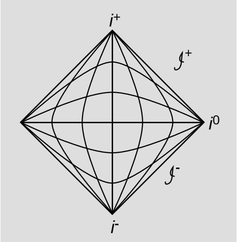
The distortion becomes greater as we move away from the center of the diagram, and becomes infinite near the edges. Because of this infinite distortion, the points i− and i+ actually represent 3-spheres. All timelike curves start at i− and end at i+, which are idealized points at infinity, like the vanishing points in perspective drawings. We can think of i+ as the “Elephants’ graveyard,” where massive particles go when they die. Similarly, lightlike curves end on \(\mathscr{I}^{+}\) (which includes its mirror image on the left), referred to as null infinity.3 The point at i0 is an infinitely distant endpoint for spacelike curves. Because of the spherical symmetry, the left and right halves of the diagram are redundant.
It is possible to make up explicit formulae that translate back and forth between Minkowski coordinates and points on the diamond, but in general this is not necessary. In fact, the utility of the diagrams is that they let us think about causal relationships in coordinate-independent ways. A light cone on the diagram looks exactly like a normal light cone.
Since this particular spacetime is homogeneous, it makes no difference what spatial location on the diagram we pick as our axis of symmetry. For example, we could arbitrarily pick the left-hand corner, the central timelike geodesic (drawn straight) or one of the other timelike geodesics (represented as if it were curved).
Schwarzschild Spacetime
Figure 7.3.2 is a Penrose diagram for the Schwarzschild spacetime, i.e., a spacetime that looks like Minkowski space, except that it has one eternal black hole in it. This is a black hole that did not form by gravitational collapse. This spacetime isn’t homogeneous; it has a specific location that is its center of spherical symmetry, and this is the vertical line on the left marked r = 0. The triangle is the spacetime inside the event horizon; we could have copied it across the r = 0 line if we had so desired, but the copies would have been redundant.
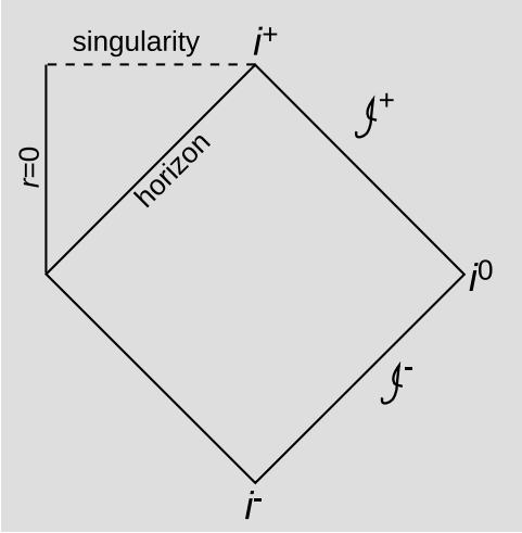
The Penrose diagram makes it easy to reason about causal relationships. For example, we can see that if a particle reaches a point inside the event horizon, its entire causal future lies inside the horizon, and all of its possible future world-lines intersect the singularity. The horizon is a lightlike surface, which makes sense, because it’s defined as the boundary of the set of points from which a light ray could reach \(\mathscr{I}^{+}\).
Astrophysical Black Hole
Figure 7.3.3 is a Penrose diagram for a black hole that has formed by gravitational collapse. Using this type of diagram, we can succinctly address one of the most vexing FAQs about black holes. (Cf. section 6.3, where we took a more cumbersome approach without Penrose diagrams.) If a distant observer watches the collapsing cloud of matter from which the black hole forms, her optical observations will show that the light from the matter becomes more and more gravitationally redshifted, and if she wishes, she can interpret this as an example of gravitational time dilation. As she waits longer and longer, the light signals from the infalling matter take longer and longer to arrive. The redshift approaches infinity as the matter approaches the horizon, so the light waves ultimately become too low in energy to be detectable by any given instrument. Furthermore, her patience (or her lifetime) will run out, because the time on her clock approaches infinity as she waits to get signals from matter that is approaching the horizon. This is all exactly as it should be, since the horizon is by definition the boundary of her observable universe. (A light ray emitted from the horizon will end up at i+, which is an end-point of timelike world-lines reached only by observers who have experienced an infinite amount of proper time.)
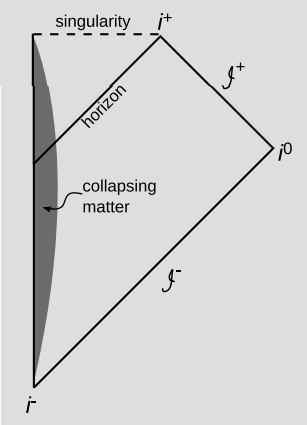
People who are bothered by these issues often acknowledge the external unobservability of matter passing through the horizon, and then want to pass from this to questions like, “Does that mean the black hole never really forms?” This presupposes that our distant observer has a uniquely defined notion of simultaneity that applies to a region of space stretching from her own position to the interior of the black hole, so that she can say what’s going on inside the black hole “now.” But the notion of simultaneity in general relativity is even more limited than its counterpart in special relativity. Not only is simultaneity in general relativity observer-dependent, as in special relativity, but it is also local rather than global.
In Figure 7.3.4, E is an event on the world-line of an observer. The spacelike surface S1 is one possible “now” for this observer. According to this surface, no particle has ever fallen in and reached the horizon; every such particle has a world-line that intersects S1, and therefore it’s still on its way in.
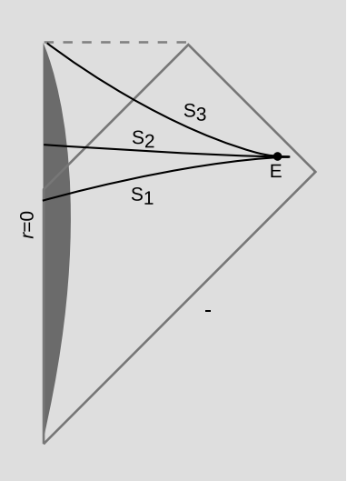
S2 is another possible “now” for the same observer at the same time. According to this definition of “now,” all the particles have passed the event horizon, but none have hit the singularity yet. Finally, S3 is a “now” according to which all the particles have hit the singularity.
If this was special relativity, then we could decide which surface was the correct notion of simultaneity for the observer, based on the observer’s state of motion. But in general relativity, this only works locally (which is why I made all three surfaces coincide near E). There is no well-defined way of deciding which is the correct way of globally extending this notion of simultaneity.
Although it may seem strange that we can’t say whether the singularity has “already” formed according to a distant observer, this is really just an inevitable result of the fact that the singularity is spacelike. The same thing happens in the case of a Schwarzschild spacetime, which we think of as a description of an eternal black hole, i.e., one that has always existed and always will. On the similar Penrose diagram for an eternal black hole, we can still draw a spacelike surface like S1 or S2, representing a definition of “now” such that the singularity doesn’t exist yet.
Penrose Diagrams in General
Ideally we would like to generalize the procedure for drawing Penrose diagrams so that we would be able to uniquely determine one for any spacetime. This turns out to be not so clear-cut. The procedure would go something like this:
- Make an n-dimensional section or projection, where usually, but not always, n = 2.
- Do a transformation to reduce the resulting manifold to a flat one of finite size.
- Adjoin idealized surfaces and points at infinity.
At step 1, we want to take advantage of any symmetries, such as rotational symmetry, so that the final result will be informative, be representative of the whole spacetime, and accurately depict causal relationships in the original spacetime. If the original spacetime has a low degree of symmetry (e.g., a spacetime containing three black holes arranged in a triangle), then this might require n > 2. At this step we also need to make sure that lightlike geodesics in the original space correspond properly to lightlike geodesics in the submanifold.
For step 2, we have already given a geometrical characterization of the type of transformation we have in mind, which is called a conformal transformation. It turns out to be possible to encapsulate this idea in a simple analytic way. Given a spacetime with a metric g, we define a fictitious metric \(\tilde{g} = \Omega^{2} g\), where \(\Omega\) is a nonzero real number that varies from point to point. (Cf. sec. 5.11, where \(\Omega\) was constant.) The idea here is that g and \(\tilde{g}\) agree on where the light cone is, but they disagree on the measurement of distances and times. The same manifold equipped with the fictitious metric \(\tilde{g}\) is the one being drawn on the page when we make a Penrose diagram. We let \(\Omega\) → 0 as we approach the idealized boundary regions like i0 and \(\mathscr{I}^{+}\), and this is what causes the Penrose diagram to take up finite space on the page.
It is not possible in general to do what is required in step 2 by making a conformal transformation to change a manifold into a flat one. A manifold that can be flattened in this way is called conformally flat. All two-dimensional manifolds are conformally flat, so in the n = 2 case this is guaranteed. For n > 3 we will usually not have conformal flatness if there are gravitational waves or tidal forces present.
The most problematic part, surprisingly, is step 3. This topic goes under the general heading of “boundary constructions.” Reviews are available on this topic.4 There are a number of more or less specific techniques for constructing a boundary, with an alphabet soup of names including the g-boundary, c-boundary, b-boundary, and a-boundary. As someone who is not a specialist in this subfield, the impression I get is that this is an area of research that has turned out badly and has never produced any useful results, but work continues, and it is possible that at some point the smoke will clear. As a simple example of what one would like to get, but doesn’t get, from these studies, it would seem natural to ask how many dimensions there are in a black hole singularity. (See example 4 for a discussion of why this is a nontrivial question.) Different answers come back from the different methods. For example, the b-boundary approach says that both black-hole and cosmological singularities are zero-dimensional points, while in the c-boundary method (which was designed to harmonize with Penrose diagrams) they are three-surfaces (as one would imagine from the Penrose diagrams).
Global Hyperbolicity
Causality refers to our vaguely defined feeling that the world should have an orderly progression of cause and effect. Making this notion more precise is surprisingly difficult. Penrose diagrams, and their associated concepts, are essentially representations of the causal structure of spacetime, and these turn out to be helpful in putting together one of the more satisfying attempts to define causality. This definition is called global hyperbolicity. The obscure terminology is related to the classification of partial differential equations.
Some definitions are required as a preliminary. Consider a set S of events in spacetime. S is bounded if it does not include any of the idealized points on the Penrose diagram that we have added at infinity.5 S is closed if it contains its own boundary.6 S is compact if it is closed and bounded.
Notes
5 More rigorously, this is equivalent to saying that for any geodesic in S, there is a bound on the affine parameter.
6 To make this more precise, we proceed as described in section 5.10 by enlarging the set of points in our spacetime manifold M to include points at infinitesimal distances from one of the original points. Then S is closed if, for any point in the enlarged version of S, there is a point lying at an infinitesimal distance from it in the original version of S.
Example 9: Compact and noncompact light cones
Figure 7.3.5 shows a spacetime containing a black hole that forms by gravitational collapse. Point P is inside the event horizon, Q outside. Consider the following four point-sets:
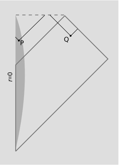
I+ (P), called the chronological future of P, is the interior of P’s future-directed light cone.
J+ (P) is like I+ (P), but also includes events that are on the boundary of the light cone, i.e., events that cannot be connected to P by a timelike curve but that can be connected to it by a lightlike curve. We call this the causal future of P, since it is the set of events that could be caused by P.
I+ (Q) and J+ (Q) are the analogous sets built on Q.
Of these four sets, only J+ (P) is compact. I+ (P) is noncompact because it is not closed. I+ (Q) and J+ (Q) are noncompact because they are not bounded; they include idealized points at infinity that lie in i+ and \(\mathscr{I}^{+}\).
In addition to the notation introduced in example 9, we will need the similar notations I− and J− for the corresponding past light-cones.
Definition
A spacetime is globally hyperbolic if: (1) there are no closed, timelike curves (CTCs),7 and (2) given any two events P and Q, the intersection of J+(P) and J−(Q) is compact. (Condition 2 is required only when P and Q are points in the manifold, not boundary points.)
7 For precision, the condition needs to be made a little stronger. We want no closed, non-spacelike curves, and we also want it to be impossible for curves to exist that are arbitrarily close to being such curves, in the sense that for any event, there exists a neighborhood around it that can never be revisited.
In a globally hyperbolic spacetime, initial-value problems always have unique solutions. That is, we can pick a spacelike surface and give the value of a wave on that surface, and the wave equation will then have a unique solution. Such a surface is called a Cauchy surface.
We can readily verify by inspection of the Penrose digrams that the spacetimes described earlier in this section are globally hyperbolic. Condition 2 implies that the intersection doesn’t contain any singularities or points at infinity. Although black hole spacetimes do contain singularities, the spacelike nature of these singularities implies that they can never lie in the intersection of light cones as referred to in the definition. Therefore such spacetimes are globally hyperbolic.
Example 10: Global hyperbolicity
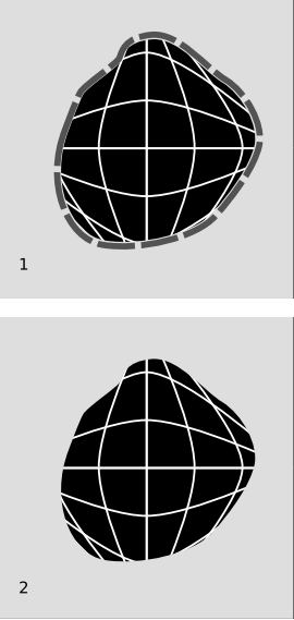
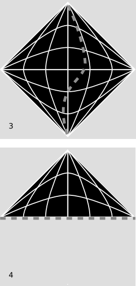
Figure 7.3.6 (1) shows a piece cut out of Minkowski space. The dashed outline is meant to indicate that the piece doesn’t include its boundary. This spacetime is not globally hyperbolic. For certain choices of events P and Q, the intersection J+ (P) ∩ J−(Q) could extend out to the cut at the edge. Since the spacetime doesn’t include its boundary, this intersection would not be compact. It’s easy to see why causality fails in this spacetime. If we pick a spacelike surface near the bottom of the diagram, it would only cut through a small part of the bottom of the spacetime. At later times, the spacetime grows at a rate that is greater than c. Therefore such a surface cannot be used as a Cauchy surface; given the initial conditions on this surface, we cannot predict what will happen in the parts of the universe that are outside its causal future.
In Figure 7.3.6 (2) we have the same example, but now the boundary is included. This set is not a manifold, which excludes it from consideration as a spacetime in general relativity. Figure 7.3.6 (3) is a picture of Minkowski space with a timelike singularity in it (dashed line). Singularities are not point-sets in the manifold, so topologically, this is like Minkowski space with a single timelike curve surgically removed. Global hyperbolicity fails because the intersection J+ (P) ∩ J−(Q) could surround the singularity, and would not be compact because it would not include its boundary at the singularity. This violation of global hyperbolicity indicates a failure of causality in such a spacetime (see section 6.3).
By cutting off the lower half of the diamond representing Minkowski spacetime, we obtain Figure 7.3.6 (4). The dashed line indicates that the boundary is not included, and therefore this is a manifold. It is also globally hyperbolic. This example suggests that global hyperbolicity does not necessarily capture everything we might ever want to describe in a definition of causality. If a paleontologist living in this spacetime finds a dinosaur fossil embedded in a rock, she will naturally infer that a dinosaur lived at some point in the past, causing the fossil to exist. But perhaps this is not the case — the hypothetical dinosaur might be one that would have existed before the boundary. This creationism-flavored violation of causality is of a different flavor than the situation we would have had if the bottom edge of the diagram had been a big bang singularity; in that case, we would have had a knowable reason why chains of cause and effect could not be extended back into the past beyond a certain time.
References
3 See also section 7.4
4 Ashley, “Singularity theorems and the abstract boundary construction,” digitalcollections.anu.edu.a...dle/1885/46055. GarciaParrado and Senovilla, “Causal structures and causal boundaries,” http:// arxiv.org/abs/gr-qc/0501069.