
13.8: Einstein's Theory of Gravity
- Page ID
- 4710

- Describe how the theory of general relativity approaches gravitation
- Explain the principle of equivalence
- Calculate the Schwarzschild radius of an object
- Summarize the evidence for black holes
Newton’s law of universal gravitation accurately predicts much of what we see within our solar system. Indeed, only Newton’s laws have been needed to accurately send every space vehicle on its journey. The paths of Earth-crossing asteroids, and most other celestial objects, can be accurately determined solely with Newton’s laws. Nevertheless, many phenomena have shown a discrepancy from what Newton’s laws predict, including the orbit of Mercury and the effect that gravity has on light. In this section, we examine a different way of envisioning gravitation.
A Revolution in Perspective
In 1905, Albert Einstein published his theory of special relativity. This theory is discussed in great detail in Relativity so we say only a few words here. In this theory, no motion can exceed the speed of light—it is the speed limit of the Universe. This simple fact has been verified in countless experiments. However, it has incredible consequences—space and time are no longer absolute. Two people moving relative to one another do not agree on the length of objects or the passage of time. Almost all of the mechanics you learned in previous chapters, while remarkably accurate even for speeds of many thousands of miles per second, begin to fail when approaching the speed of light.
This speed limit on the Universe was also a challenge to the inherent assumption in Newton’s law of gravitation that gravity is an action-at-a-distance force. That is, without physical contact, any change in the position of one mass is instantly communicated to all other masses. This assumption does not come from any first principle, as Newton’s theory simply does not address the question. (The same was believed of electromagnetic forces, as well. It is fair to say that most scientists were not completely comfortable with the action-at-a-distance concept.)
A second assumption also appears in Newton’s law of gravitation Equation 13.2.1. The masses are assumed to be exactly the same as those used in Newton’s second law, \(\vec{F}\) = m\(\vec{a}\). We made that assumption in many of our derivations in this chapter. Again, there is no underlying principle that this must be, but experimental results are consistent with this assumption. In Einstein’s subsequent theory of general relativity (1916), both of these issues were addressed. His theory was a theory of space-time geometry and how mass (and acceleration) distort and interact with that space-time. It was not a theory of gravitational forces. The mathematics of the general theory is beyond the scope of this text, but we can look at some underlying principles and their consequences.
The Principle of Equivalence
Einstein came to his general theory in part by wondering why someone who was free falling did not feel his or her weight. Indeed, it is common to speak of astronauts orbiting Earth as being weightless, despite the fact that Earth’s gravity is still quite strong there. In Einstein’s general theory, there is no difference between free fall and being weightless. This is called the principle of equivalence. The equally surprising corollary to this is that there is no difference between a uniform gravitational field and a uniform acceleration in the absence of gravity. Let’s focus on this last statement. Although a perfectly uniform gravitational field is not feasible, we can approximate it very well.
Within a reasonably sized laboratory on Earth, the gravitational field \(\vec{g}\) is essentially uniform. The corollary states that any physical experiments performed there have the identical results as those done in a laboratory accelerating at \(\vec{a} = \vec{g}\) in deep space, well away from all other masses. Figure \(\PageIndex{1}\) illustrates the concept.
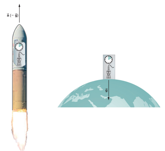
How can these two apparently fundamentally different situations be the same? The answer is that gravitation is not a force between two objects but is the result of each object responding to the effect that the other has on the space-time surrounding it. A uniform gravitational field and a uniform acceleration have exactly the same effect on space-time.
A Geometric Theory of Gravity
Euclidian geometry assumes a “flat” space in which, among the most commonly known attributes, a straight line is the shortest distance between two points, the sum of the angles of all triangles must be 180 degrees, and parallel lines never intersect. Non-Euclidean geometry was not seriously investigated until the nineteenth century, so it is not surprising that Euclidean space is inherently assumed in all of Newton’s laws.
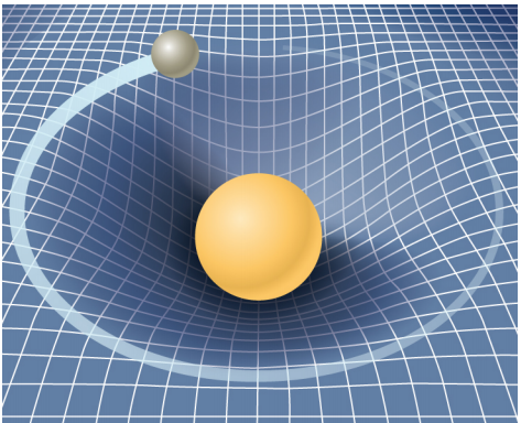
The general theory of relativity challenges this long-held assumption. Only empty space is flat. The presence of mass—or energy, since relativity does not distinguish between the two—distorts or curves space and time, or space-time, around it. The motion of any other mass is simply a response to this curved space-time. Figure \(\PageIndex{2}\) is a two-dimensional representation of a smaller mass orbiting in response to the distorted space created by the presence of a larger mass. In a more precise but confusing picture, we would also see space distorted by the orbiting mass, and both masses would be in motion in response to the total distortion of space. Note that the figure is a representation to help visualize the concept. These are distortions in our three-dimensional space and time. We do not see them as we would a dimple on a ball. We see the distortion only by careful measurements of the motion of objects and light as they move through space.
For weak gravitational fields, the results of general relativity do not differ significantly from Newton’s law of gravitation. But for intense gravitational fields, the results diverge, and general relativity has been shown to predict the correct results. Even in our Sun’s relatively weak gravitational field at the distance of Mercury’s orbit, we can observe the effect. Starting in the mid-1800s, Mercury’s elliptical orbit has been carefully measured. However, although it is elliptical, its motion is complicated by the fact that the perihelion position of the ellipse slowly advances. Most of the advance is due to the gravitational pull of other planets, but a small portion of that advancement could not be accounted for by Newton’s law. At one time, there was even a search for a “companion” planet that would explain the discrepancy. But general relativity correctly predicts the measurements. Since then, many measurements, such as the deflection of light of distant objects by the Sun, have verified that general relativity correctly predicts the observations.
We close this discussion with one final comment. We have often referred to distortions of space-time or distortions in both space and time. In both special and general relativity, the dimension of time has equal footing with each spatial dimension (differing in its place in both theories only by an ultimately unimportant scaling factor). Near a very large mass, not only is the nearby space “stretched out,” but time is dilated or “slowed.” We discuss these effects more in the next section.
Black Holes
Einstein’s theory of gravitation is expressed in one deceptively simple-looking tensor equation (tensors are a generalization of scalars and vectors), which expresses how a mass determines the curvature of space-time around it. The solutions to that equation yield one of the most fascinating predictions: the black hole. The prediction is that if an object is sufficiently dense, it will collapse in upon itself and be surrounded by an event horizon from which nothing can escape. The name “black hole,” which was coined by astronomer John Wheeler in 1969, refers to the fact that light cannot escape such an object. Karl Schwarzschild was the first person to note this phenomenon in 1916, but at that time, it was considered mostly to be a mathematical curiosity.
Surprisingly, the idea of a massive body from which light cannot escape dates back to the late 1700s. Independently, John Michell and Pierre Simon Laplace used Newton’s law of gravitation to show that light leaving the surface of a star with enough mass could not escape. Their work was based on the fact that the speed of light had been measured by Ole Roemer in 1676. He noted discrepancies in the data for the orbital period of the moon Io about Jupiter. Roemer realized that the difference arose from the relative positions of Earth and Jupiter at different times and that he could find the speed of light from that difference. Michell and Laplace both realized that since light had a finite speed, there could be a star massive enough that the escape speed from its surface could exceed that speed. Hence, light always would fall back to the star. Oddly, observers far enough away from the very largest stars would not be able to see them, yet they could see a smaller star from the same distance.
Recall that in Gravitational Potential Energy and Total Energy, we found that the escape speed, given by \(v_{\mathrm{esc}}=\sqrt{\frac{2 G M}{R}}\), is independent of the mass of the object escaping. Even though the nature of light was not fully understood at the time, the mass of light, if it had any, was not relevant. Hence, this equation should be valid for light. Substituting c, the speed of light, for the escape velocity, we have
\[v_{esc} = c = \sqrt{\dfrac{2GM}{R}} \ldotp\]
Thus, we only need values for R and M such that the escape velocity exceeds c, and then light will not be able to escape. Michell posited that if a star had the density of our Sun and a radius that extended just beyond the orbit of Mars, then light would not be able to escape from its surface. He also conjectured that we would still be able to detect such a star from the gravitational effect it would have on objects around it. This was an insightful conclusion, as this is precisely how we infer the existence of such objects today. While we have yet to, and may never, visit a black hole, the circumstantial evidence for them has become so compelling that few astronomers doubt their existence.
Before we examine some of that evidence, we turn our attention back to Schwarzschild’s solution to the tensor equation from general relativity. In that solution arises a critical radius, now called the Schwarzschild radius (RS). For any mass M, if that mass were compressed to the extent that its radius becomes less than the Schwarzschild radius, then the mass will collapse to a singularity, and anything that passes inside that radius cannot escape. Once inside RS, the arrow of time takes all things to the singularity. (In a broad mathematical sense, a singularity is where the value of a function goes to infinity. In this case, it is a point in space of zero volume with a finite mass. Hence, the mass density and gravitational energy become infinite.) The Schwarzschild radius is given by
\[R_{S} = \dfrac{2GM}{c^{2}} \ldotp \label{13.12}\]
If you look at our escape velocity equation with vesc = c, you will notice that it gives precisely this result. But that is merely a fortuitous accident caused by several incorrect assumptions. One of these assumptions is the use of the incorrect classical expression for the kinetic energy for light. Just how dense does an object have to be in order to turn into a black hole?
Calculate the Schwarzschild radius for both the Sun and Earth. Compare the density of the nucleus of an atom to the density required to compress Earth’s mass uniformly to its Schwarzschild radius. The density of a nucleus is about 2.3 x 10¹⁷ kg/m3.
Strategy
We use Equation \ref{13.12} for this calculation. We need only the masses of Earth and the Sun, which we obtain from the astronomical data given in Appendix D.
Solution
Substituting the mass of the Sun, we have
\[R_{S} = \dfrac{2GM}{c^{2}} = \dfrac{2(6.67 \times 10^{-11}\; N\; \cdotp m^{2}/kg^{2})(1.99 \times 10^{30}\; kg)}{(3.0 \times 10^{8}\; m/s)^{2}} = 2.95 \times 10^{3}\; m \ldotp\]
This is a diameter of only about 6 km. If we use the mass of Earth, we get RS = 8.85 x 10⁻³ m. This is a diameter of less than 2 cm! If we pack Earth’s mass into a sphere with the radius RS = 8.85 x 10⁻³ m, we get a density of
\[\rho = \dfrac{mass}{volume} = \dfrac{5.97 \times 10^{24}\; kg}{\dfrac{4}{3} \pi (8.85 \times 10^{-3}\; m)^{3}} = 2.06 \times 10^{30}\; kg/m^{3} \ldotp\]
Significance
A neutron star is the most compact object known—outside of a black hole itself. The neutron star is composed of neutrons, with the density of an atomic nucleus, and, like many black holes, is believed to be the remnant of a supernova—a star that explodes at the end of its lifetime. To create a black hole from Earth, we would have to compress it to a density thirteen orders of magnitude greater than that of a neutron star. This process would require unimaginable force. There is no known mechanism that could cause an Earth-sized object to become a black hole. For the Sun, you should be able to show that it would have to be compressed to a density only about 80 times that of a nucleus. (Note: Once the mass is compressed within its Schwarzschild radius, general relativity dictates that it will collapse to a singularity. These calculations merely show the density we must achieve to initiate that collapse.)
Consider the density required to make Earth a black hole compared to that required for the Sun. What conclusion can you draw from this comparison about what would be required to create a black hole? Would you expect the Universe to have many black holes with small mass?
The Event Horizon
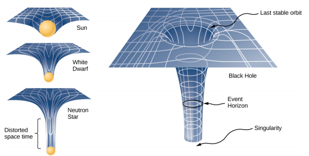
The Schwarzschild radius is also called the event horizon of a black hole. We noted that both space and time are stretched near massive objects, such as black holes. Figure \(\PageIndex{3}\) illustrates that effect on space. The distortion caused by our Sun is actually quite small, and the diagram is exaggerated for clarity. Consider the neutron star, described in Example \(\PageIndex{1}\). Although the distortion of space-time at the surface of a neutron star is very high, the radius is still larger than its Schwarzschild radius. Objects could still escape from its surface.
However, if a neutron star gains additional mass, it would eventually collapse, shrinking beyond the Schwarzschild radius. Once that happens, the entire mass would be pulled, inevitably, to a singularity. In the diagram, space is stretched to infinity. Time is also stretched to infinity. As objects fall toward the event horizon, we see them approaching ever more slowly, but never reaching the event horizon. As outside observers, we never see objects pass through the event horizon—effectively, time is stretched to a stop.
Visit this site to view an animated example of these spatial distortions.
The evidence for black holes
Not until the 1960s, when the first neutron star was discovered, did interest in the existence of black holes become renewed. Evidence for black holes is based upon several types of observations, such as radiation analysis of X-ray binaries, gravitational lensing of the light from distant galaxies, and the motion of visible objects around invisible partners. We will focus on these later observations as they relate to what we have learned in this chapter. Although light cannot escape from a black hole for us to see, we can nevertheless see the gravitational effect of the black hole on surrounding masses.
The closest, and perhaps most dramatic, evidence for a black hole is at the center of our Milky Way galaxy. The UCLA Galactic Group, using data obtained by the W. M. Keck telescopes, has determined the orbits of several stars near the center of our galaxy. Some of that data is shown in Figure \(\PageIndex{4}\). The orbits of two stars are highlighted. From measurements of the periods and sizes of their orbits, it is estimated that they are orbiting a mass of approximately 4 million solar masses. Note that the mass must reside in the region created by the intersection of the ellipses of the stars. The region in which that mass must reside would fit inside the orbit of Mercury—yet nothing is seen there in the visible spectrum.
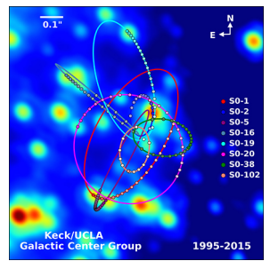
The physics of stellar creation and evolution is well established. The ultimate source of energy that makes stars shine is the self-gravitational energy that triggers fusion. The general behavior is that the more massive a star, the brighter it shines and the shorter it lives. The logical inference is that a mass that is 4 million times the mass of our Sun, confined to a very small region, and that cannot be seen, has no viable interpretation other than a black hole. Extragalactic observations strongly suggest that black holes are common at the center of galaxies.
Visit the UCLA Galactic Center Group main page for information on X-ray binaries and gravitational lensing. Visit this page to view a three-dimensional visualization of the stars orbiting near the center of our galaxy, where the animation is near the bottom of the page.
Dark Matter
Stars orbiting near the very heart of our galaxy provide strong evidence for a black hole there, but the orbits of stars far from the center suggest another intriguing phenomenon that is observed indirectly as well. Recall from Gravitation Near Earth’s Surface that we can consider the mass for spherical objects to be located at a point at the center for calculating their gravitational effects on other masses. Similarly, we can treat the total mass that lies within the orbit of any star in our galaxy as being located at the center of the Milky Way disc. We can estimate that mass from counting the visible stars and include in our estimate the mass of the black hole at the center as well.
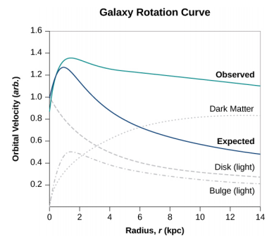
But when we do that, we find the orbital speed of the stars is far too fast to be caused by that amount of matter. Figure \(\PageIndex{5}\) shows the orbital velocities of stars as a function of their distance from the center of the Milky Way. The blue line represents the velocities we would expect from our estimates of the mass, whereas the green curve is what we get from direct measurements. Apparently, there is a lot of matter we don’t see, estimated to be about five times as much as what we do see, so it has been dubbed dark matter. Furthermore, the velocity profile does not follow what we expect from the observed distribution of visible stars. Not only is the estimate of the total mass inconsistent with the data, but the expected distribution is inconsistent as well. And this phenomenon is not restricted to our galaxy, but seems to be a feature of all galaxies. In fact, the issue was first noted in the 1930s when galaxies within clusters were measured to be orbiting about the center of mass of those clusters faster than they should based upon visible mass estimates.
There are two prevailing ideas of what this matter could be—WIMPs and MACHOs. WIMPs stands for weakly interacting massive particles. These particles (neutrinos are one example) interact very weakly with ordinary matter and, hence, are very difficult to detect directly. MACHOs stands for massive compact halo objects, which are composed of ordinary baryonic matter, such as neutrons and protons. There are unresolved issues with both of these ideas, and far more research will be needed to solve the mystery.