27A: Oscillations: Introduction, Mass on a Spring

If a simple harmonic oscillation problem does not involve the time, you should probably be using conservation of energy to solve it. A common “tactical error” in problems involving oscillations is to manipulate the equations giving the position and velocity as a function of time, \(x=x_{\space max} cos(2\pi ft)\) and \(v=-v_{\space max} sin(2\pi ft)\) rather than applying the principle of conservation of energy. This turns an easy five-minute problem into a difficult fifteen-minute problem.

When something goes back and forth we say it vibrates or oscillates. In many cases oscillations involve an object whose position as a function of time is well characterized by the sine or cosine function of the product of a constant and elapsed time. Such motion is referred to as sinusoidal oscillation. It is also referred to as simple harmonic motion.

Math Aside: The Cosine Function

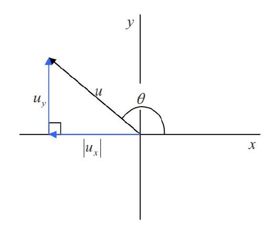
By now, you have had a great deal of experience with the cosine function of an angle as the ratio of the adjacent to the hypotenuse of a right triangle. This definition covers angles from 0 radians to \(\frac{\pi}{2}\) radians (\(0^{\circ}\) to \(90^{\circ}\)). In applying the cosine function to simple harmonic motion, we use the extended definition which covers all angles. The extended definition of the cosine of the angle \(\theta\) is that the cosine of an angle is the x component of a unit vector, the tail of which is on the origin of an x-y coordinate system; a unit vector that originally pointed in the +x direction but has since been rotated counterclockwise from our viewpoint, through the angle \(\theta\), about the origin.

Here we show that the extended definition is consistent with the “adjacent over hypotenuse” definition, for angles between 0 radians and \(\frac{\pi}{2}\) radians. For such angles, we have:

in which, \(u\), being the magnitude of a unit vector, is of course equal to 1, the pure number 1 with no units. Now, according to the ordinary definition of the cosine of \(\theta\) as the adjacent over the hypotenuse:

\[\cos\space \theta=\space \frac{u_x}{u} \nonumber \]

Solving this for \(u_x\) we see that

\[u_x=u \, \cos\theta \nonumber \]

Recalling that \(u=1\), this means that

\[u_x=\space \cos\theta \nonumber \]

Recalling that our extended definition of \(\cos \theta\) is, that it is the x component of the unit vector \(\hat{u}\) when \(\hat{u}\) makes an angle \(\theta\) with the x-axis, this last equation is just saying that, for the case at hand ( \(\theta \) between 0 and \(\frac{\pi}{2}\) ) our extended definition of \(\cos \theta\) is equivalent to our ordinary definition.

At angles between \(\frac{\pi}{2}\) and \(\frac{3\pi}{2}\) radians ( \(90^{\circ}\) and \(270^{\circ}\) ) we see that \(u_x\) takes on negative values (when the x component vector is pointing in the negative x direction, the x component value is, by definition, negative). According to our extended definition, \(\cos \theta\) takes on negative values at such angles as well.

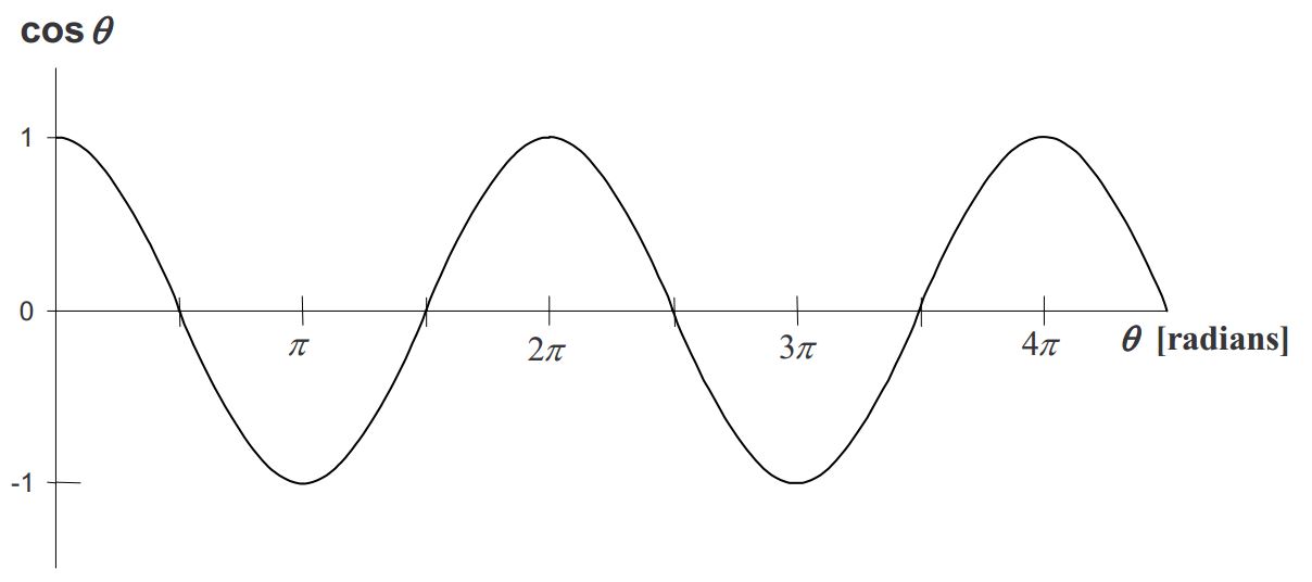
With our extended definition, valid for any angle \(\theta\), a graph of the \(\cos \theta\) vs. \(\theta\) appears as:

Some Calculus Relations Involving the Cosine

The derivative of the cosine of \(\theta\), with respect to \(\theta\):

\[ \frac{d}{d\theta} \cos\theta \space=\space -\sin\theta \nonumber \]

The derivative of the sine of \(\theta\), with respect to \(\theta\):

\[ \frac{d}{d\theta} \sin\theta \space=\space \cos\theta \nonumber \]

Some Jargon Involving The Sine And Cosine Functions

When you express, define, or evaluate the function of something, that something is called the argument of the function. For instance, suppose the function is the square root function and the expression in question is \(\sqrt{3x}\). The expression is the square root of \(3x\), so, in \(x\) that expression, \(3x\) is the argument of the square root function. Now when you take the cosine of something, that something is called the argument of the cosine, but in the case of the sine and cosine functions, we give it another name as well, namely, the phase. So, when you write \(\cos \theta\), the variable \(\theta\) is the argument of the cosine function, but it is also referred to as the phase of the cosine function.In order for an expression involving the cosine function to be at all meaningful, the phase of the cosine must have units of angle (for instance, radians or degrees).

A Block Attached to the End of a Spring

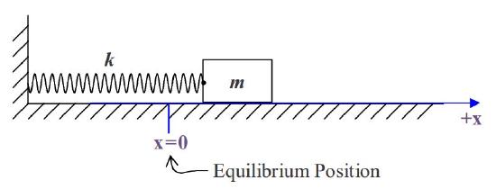
Consider a block of mass \(m\) on a frictionless horizontal surface. The block is attached, by means of an ideal massless horizontal spring having force constant \(k\), to a wall. A person has pulled the block out, directly away from the wall, and released it from rest. The block oscillates back and forth (toward and away from the wall), on the end of the spring. We would like to find equations that give the block’s position, velocity, and acceleration as functions of time. We start by applying Newton’s 2^nd Law to the block. Before drawing the free body diagram we draw a sketch to help identify our one-dimensional coordinate system. We will call the horizontal position of the point at which the spring is attached, the position \(x\) of the block. The origin of our coordinate system will be the position at which the spring is neither stretched nor compressed. When the position \(x\) is positive, the spring is stretched and exerts a force, on the block, in the \(-x\) direction. When the position of \(x\) is negative, the spring is compressed and exerts a force, on the block, in the \(+x\) direction.

Now we draw the free body diagram of the block:

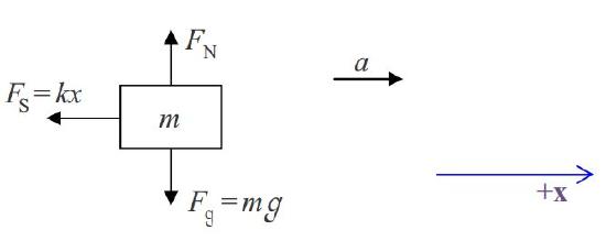
and apply Newton’s 2^nd Law:

\[a_{\rightarrow}=\frac{1}{m} \sum F_{\rightarrow} \nonumber \]

\[a=\frac{1}{m}(-kx) \nonumber \]

\[a=-\frac{k}{m}x \nonumber \]

This equation, relating the acceleration of the block to its position x, can be considered to be an equation relating the position of the block to time if we substitute for a using:

\[a\space=\space \frac{dv}{dt} \nonumber \]

and

\[v\space=\space \frac{dx}{dt} \nonumber \]

so

\[a=\frac{d}{dt}\space \frac{dx}{dt} \nonumber \]

which is usually written

\[a=\space \frac{d^2x}{dt^2}\label{27-1} \]

and read “\(d\) squared \(x\) by \(dt\) squared” or “the second derivative of \(x\) with respect to \(t\).”

Substituting this expression for \(a\) into \(a=-\frac{k}{m} x\) (the result we derived from Newton’s 2^nd Law above) yields

\[\frac{d^2x}{dt^2}=-\frac{k}{m}x\label{27-2} \]

We know in advance that the position of the block depends on time. That is to say, \(x\) is a function of time. This equation, equation \(\ref{27-2}\), tells us that if you take the second derivative of \(x\) with respect to time you get \(x\) itself, times a negative constant \((-k/m)\).

We can find the an expression for x in terms of t that solves \(\ref{27-2}\) by the method of “guess and check.” Grossly, we’re looking for a function whose second derivative is essentially the negative of itself. Two functions meet this criterion, the sine and the cosine. Either will work. We arbitrarily choose to use the cosine function. We include some constants in our trial solution (our guess) to be determined during the “check” part of our procedure. Here’s our trial solution:

\[x= x_{max} \, \cos \left(\frac{2\pi\space \mbox{rad}}{T}t\right) \nonumber \]

Here’s how we have arrived at this trial solution: Having established that x, depends on the cosine of a multiple of the time variable, we let the units be our guide. We need the time t to be part of the argument of the cosine, but we can’t take the cosine of something unless that something has units of angle. The constant \(\frac{2\pi\space \mbox{rad}}{T}\), with the constant T having units of time (we’ll use seconds), makes it so that the argument of the cosine has units of radians. It is, however, more than just the units that motivates us to choose the ratio \(\frac{2\pi\space \mbox{rad}}{T}\) as the constant. To make the argument of the cosine have units of radians, all we need is a constant with units of radians per second. So why write it as \(\frac{2\pi\space \mbox{rad}}{T}\)? Here’s the explanation: The block goes back and forth. That is, it repeats its motion over and over again as time goes by. Starting with the block at its maximum distance from the wall, the block moves toward the wall, reaches its closest point of approach to the wall and then comes back out to its maximum distance from the wall. At that point, it’s right back where it started from. We define the constant value of time \(T\) to be the amount of time that it takes for one iteration of the motion.

Now consider the cosine function. We chose it because its second derivative is the negative of itself, but it is looking better and better as a function that gives the position of the block as a function of time because it too repeats itself as its phase (the argument of the cosine) continually increases. Suppose the phase starts out as 0 at time 0. The cosine of 0 radians is 1, the biggest the cosine ever gets. We can make this correspond to the block being at its maximum distance from the wall. As the phase increases, the cosine gets smaller, then goes negative, eventually reaching the value -1 when the phase is π radians. This could correspond to the block being closest to the wall. Then, as the phase continues to increase, the cosine increases until, when the phase is \(2\pi\), the cosine is back up to 1 corresponding to the block being right back where it started from. From here, as the phase of the cosine continues to increase from \(2\pi\) to \(4\pi\), the cosine again takes on all the values that it took on from 0 to \(2\pi\). The same thing happens again as the phase increases from \(4\pi\) to \(6\pi\), from \(8\pi\) to \(10\pi\), etc.

Getting back to that constant \(\frac{2\pi\space \mbox{rad}}{T}\) that we “guessed” should be in the phase of the cosine in our trial solution for \(x(t)\):

\[x= x_{max} \, \cos\Big (\frac{2\pi\space \mbox{rad}}{T}t \Big ) \nonumber \]

With \(T\) being defined as the time it takes for the block to go back and forth once, look what happens to the phase of the cosine as the stopwatch reading continually increases. Starting from 0, as t increases from 0 to \(T\), the phase of the cosine, \(\frac{2\pi\space \mbox{rad}}{T}t\), increases from 0 to \(2\pi\) radians. So, just as the block, from time 0 to time \(T\), goes though one cycle of its motion, the cosine, from time 0 to time \(T\), goes through one cycle of its pattern. As the stopwatch reading increases from \(T\) to \(2T\), the phase of the cosine increases from \(2\pi\) rad to \(4\pi\) rad. The block undergoes the second cycle of its motion and the cosine function used to determine the position of the block goes through the second cycle of its pattern. The idea holds true for any time t —as the stopwatch reading continues to increase, the cosine function keeps repeating its cycle in exact synchronization with the block, as it must if its value is to accurately represent the position of the block as a function of time. Again, it is no coincidence. We chose the constant \(\frac{2\pi\space \mbox{rad}}{T}\) in the phase of the cosine so that things would work out this way.

A few words on jargon are in order before we move on. The time \(T\) that it takes for the block to complete one full cycle of its motion is referred to as the period of the oscillations of the block. Now how about that other constant, the “\(x_{\max}\)” in our educated guess \(x= x_{\max} \, \cos \Big (\frac{2\pi\space \mbox{rad}}{T}t \Big )\)? Again, the units were our guide. When you take the cosine of an angle, you get a pure number, a value with no units. So, we need the \(x_{\max}\) there to give our function units of distance (we’ll use meters). We can further relate \(x_{\max}\) to the motion of the block. The biggest the cosine of the phase can ever get is 1, thus, the biggest \(x_{\max}\) times the cosine of the phase can ever get is \(x_{\max}\). So, in the expression \(x= x_{\max} \, \cos(\frac{2\pi\space \mbox{rad}}{T}t)\), with x being the position of the block at any time t, \(x_{\max}\) must be the maximum position of the block, the position of the block, relative to its equilibrium position, when it is as far from the wall as it ever gets.

Okay, we’ve given a lot of reasons why \(x= x_{max} \, cos(\frac{2\pi\space \mbox{rad}}{T}t)\) should well describe the motion of the block, but unless it is consistent with Newton’s 2^nd Law, that is, unless it satisfies equation \(\ref{27-2}\):

\[\frac{d^x}{dt^2}=-\frac{k}{m} x \nonumber \]

which we derived from Newton’s 2^nd Law, it is no good. So, let’s plug it into equation \(\ref{27-2}\) and see if it works. First, let’s take the second derivative \(\frac{d^2x}{dt^2}\) of our trial solution with respect to t (so we can plug it and x itself directly into equation \(\ref{27-2}\)):

Given

\[x= x_{\max} \, \cos(\frac{2\pi\space rad}{T}t) , \nonumber \]

the first derivative is

\[\frac{dx}{dt}=x_{\max} \space [ -\sin(\frac{2\pi \, \mbox{rad}}{T}t)] \frac{2\pi \, \mbox{rad}}{T} \nonumber \]

\[\frac{dx}{dt}=\space -\frac{2\pi \, \mbox{rad}}{T} \, x_{\max} \sin(\frac{2\pi \, \mbox{rad}}{T}t) \nonumber \]

The second derivative is then

\[\frac{d^2x}{dt^2}=\space -\frac{2\pi \, \mbox{rad}}{T} \, x_{\max} \cos(\frac{2\pi \, \mbox{rad}}{T}t)\frac{2\pi \, \mbox{rad}}{T}t \nonumber \]

\[\frac{d^2x}{dt^2}=\space -(\frac{2\pi \, \mbox{rad}}{T})^2 \, x_{\max} \cos(\frac{2\pi \, \mbox{rad}}{T}t) \nonumber \]

Now we are ready to substitute this and \(x\) itself, \(x=x_{\max}\space \cos(\frac{2\pi\space \mbox{rad}}{T}t)\), into the differential equation \(\frac{d^2x}{dt^2}=-\frac{k}{m}x\) (equation \(\ref{27-2}\)) stemming from Newton’s 2nd Law of Motion. The substitution yields:

\[-(\frac{2\pi \, \mbox{rad}}{T})^2 \, x_{\max} \, \cos(\frac{2\pi \, \mbox{rad} }{T}t)=-\frac{k}{m}x_{\max} \, \cos(\frac{2\pi \, \mbox{rad}}{T}t) \nonumber \]

which we copy here for your convenience.

\[-\Big (\frac{2\pi\space \mbox{rad}}{T} \Big )^2 \, x_{max} \, \cos \Big (\frac{2\pi \, \mbox{rad} }{T}t \Big) =-\frac{k}{m}x_{max} \, \cos\Big (\frac{2\pi \, \mbox{rad}}{T}t\Big ) \nonumber \]

The two sides are the same, by inspection, except that where \((\frac{2\pi\space \mbox{rad}}{T})^2\) appears on the left, we have \(\frac{k}{m}\) on the right. Thus, substituting our guess, \(x=x_{\max} \, \cos \Big (\frac{2 \pi\space \mbox{rad}}{T}t \Big )\), into the differential equation that we are trying to solve, \(\frac{d^2x}{dt^2}=-\frac{k}{m}x\) (equation \(\ref{27-2}\)) leads to an identity if and only if \( \Big (\frac{2\pi\space \mbox{rad}}{T} \Big )^2=\frac{k}{m}\). This means that the period \(T\) is determined by the characteristics of the spring and the block, more specifically by the force constant (the “stiffness factor”) \(k\) of the spring, and the mass (the inertia) of the block. Let’s solve for \(T\) in terms of these quantities. From \((\frac{2\pi\space \mbox{rad}}{T})^2=\frac{k}{m}\) we find:

\[\frac{2\pi\space \mbox{rad}}{T}=\sqrt{\frac{k}{m}} \nonumber \]

\[T=2\pi \, \mbox{rad} \sqrt{\frac{m}{k}} \nonumber \]

\[T=2\pi \sqrt{\frac{m}{k}}\label{27-3} \]

where we have taken advantage of the fact that a radian is, by definition, 1 m/m by simply deleting the “rad” from our result.

The presence of the \(m\) in the numerator means that the greater the mass, the longer the period. That makes sense: we would expect the block to be more “sluggish” when it has more mass. On the other hand, the presence of the \(k\) in the denominator means that the stiffer the spring, the shorter the period. This makes sense too in that we would expect a stiff spring to result in quicker oscillations. Note the absence of \(x_{\max}\) in the result for the period \(T\). Many folks would expect that the bigger the oscillations, the longer it would take the block to complete each oscillation, but the absence of \(x_{\max}\) in our result for \(T\) shows that it just isn’t so. The period \(T\) does not depend on the size of the oscillations.

So, our end result is that a block of mass \(m\), on a frictionless horizontal surface, a block that is attached to a wall by an ideal massless horizontal spring, and released, at time \(t=0\), from rest, from a position \(x = x_{\max}\), a distance \(x_{\max}\) from its equilibrium position; will oscillate about the equilibrium position with a period \(T=2\pi \sqrt{\frac{m}{k}}\). Furthermore, the block’s position as a function of time will be given by

\[x=x_{\max}\space \cos \Big (\frac{2\pi\space \mbox{rad}}{T}t \Big )\label{27-4} \]

From this expression for \(x(t)\) we can derive an expression for the velocity \(v(t)\) as follows:

\[v=\frac{dx}{dt} \nonumber \]

\[v=\frac{d}{dt} \Big [x_{\max} \, \cos(\frac{2\pi \, \mbox{rad}}{T}t) \Big ] \nonumber \]

\[x=x_{\max}\Big [-\sin \Big (\frac{2\pi \, \mbox{rad}}{T}t \Big )\Big ] \frac{2\pi\space \mbox{rad}}{T} \nonumber \]

\[x=-x_{\max}\frac{2\pi \, \mbox{rad}}{T} \sin \Big (\frac{2\pi \, \mbox{rad}}{T}t \Big )\label{27-5} \]

And from this expression for \(v\space (t)\) we can get the acceleration \(a\space (t)\) as follows:

\[a=\frac{dv}{dt} \nonumber \]

\[a=\frac{d}{dt} \Big [-x_{\max} \frac{2\pi \, \mbox{rad}}{T} \sin \Big (\frac{2\pi \, \mbox{rad}}{T}t \Big ) \Big ] \nonumber \]

\[a=-x_{\max}\space \frac{2\pi \, \mbox{rad}}{T} \Big [ \cos \Big( \frac{2\pi\space \mbox{rad}d}{T}t \Big) \Big] \frac{2\pi \, \mbox{rad}}{T} \nonumber \]

\[a=-x_{\max}=\Big( \frac{2\pi\space \mbox{rad}}{T} \Big)^2 \cos \Big( \frac{2\pi\space \mbox{rad}}{T}t \Big)\label{27-6} \]

Note that this latter result is consistent with the relation \(a=-\frac{k}{m}x\) between \(a\) and \(x\) that we derived from Newton’s 2^nd Law near the start of this chapter. Recognizing that the \(x_{\max}\space \cos \Big( \frac{2\pi\space \mbox{rad}}{T}t \Big)\) is \(x\) and that the \(\Big(\frac{2\pi\space \mbox{rad}}{T}\Big)^2\) is \(\frac{k}{m}\), it is clear that equation \(\ref{27-6}\) is the same thing as

\[a=-\frac{k}{m}x\label{27-7} \]

Frequency

The period \(T\) has been defined to be the time that it takes for one complete oscillation. In SI units we can think of it as the number of seconds per oscillation. The reciprocal of \(T\) is thus the number of oscillations per second. This is the rate at which oscillations occur. We give it a name, frequency, and a symbol, \(f\).

\[f=\frac{1}{T}\label{27-8} \]

The units work out to be \(\frac{1}{s}\) which we can think of as \(\frac{\mbox{oscillations}}{s}\) as the oscillation, much like the radian is a marker rather than a true unit. A special name has been assigned to the SI unit of frequency, \(1\frac{\mbox{oscillations}}{s}\) is defined to be 1 hertz, abbreviated 1 Hz. You can think of 1 Hz as either \(1\frac{\mbox{oscillations}}{s}\) or simply \(1\frac{1}{s}\).

In terms of frequency, rather than period, we can use \(f=\frac{1}{T}\) to express all our previous results in terms of \(f\) rather than \(t\).

\[f=\frac{1}{2\pi}\sqrt{\frac{k}{m}} \nonumber \]

\[x=x_{\max} \, \cos \Big(2\pi\space \mbox{rad} \space f\space t \Big) \nonumber \]

\[v=-2\pi f x_{\max} \, \sin \Big(2\pi\space \mbox{rad} \space f\space t \Big) \nonumber \]

\[a=-(2\pi f)^2 \cos \Big( 2\pi\space \mbox{rad} \space f \, t\Big) \nonumber \]

By inspection of the expressions for the velocity and acceleration above we see that the greatest possible value for the velocity is \(2\pi f x_{\max}\) and the greatest possible value for the acceleration is \((2\pi f)^2 x_{\max}\). Defining

\[v_{\max}=\space x_{\max} (2\pi f)\label{27-9} \]

and

\[a_{\max}=x_{\max} (2\pi f)^2\label{27-10} \]

and, omitting the units “rad” from the phase (thus burdening the user with remembering that the units of the phase are radians while making the expressions a bit more concise) we have:

\[x=x_{\max} \, \cos(2\pi f\space t)\label{27-11} \]

\[v=-v_{\max}\space \sin(2\pi f\space t)\label{27-12} \]

\[a=-a_{\max} \, \cos(2\pi f\space t)\label{27-13} \]

The Simple Harmonic Equation

When the motion of an object is sinusoidal as in \(x=x_{max}\space \cos (2\pi f\space t)\), we refer to the motion as simple harmonic motion. In the case of a block on a spring we found that

\[ a=-\Big| \mbox{constant} \Big|\space x\label{27-14} \]

where the \(\Big| \mbox{constant} \Big|\) was \(\frac{k}{m}\) and was shown to be equal to \((2\pi\space f)^2\). Written as

\[ \frac{d^2x}{dt^2}=-(2\pi\space f)^2 \, x\label{27-15} \]

the equation is a completely general equation, not specific to a block on a spring. Indeed, any time you find that, for any system, the second derivative of the position variable, with respect to time, is equal to a negative constant times the position variable itself, you are dealing with a case of simple harmonic motion, and you can equate the absolute value of the constant to \((2\pi\space f)^2\).