10.4: Identical Particles- Symmetry and Scattering

Introduction

For two identical particles confined to a one-dimensional box, we established earlier that the normalized two-particle wavefunction \(\psi(x_1,x_2)\), which gives the probability of finding simultaneously one particle in an infinitesimal length \(dx_1\) at \(x_1\) and another in \(dx_2\) at \(x_2\) as \(|\psi(x_1,x_2)|^2dx_1dx_2\), only makes sense if \(|\psi(x_1,x_2)|^2=|\psi(x_2,x_1)|^2\), since we don’t know which of the two indistinguishable particles we are finding where. It follows from this that there are two possible wave function symmetries: \(\psi(x_1,x_2)=\psi(x_2,x_1)\) or \(\psi(x_1,x_2)=-\psi(x_2,x_1)\). It turns out that if two identical particles have a symmetric wave function in some state, particles of that type always have symmetric wave functions, and are called bosons. (If in some other state they had an antisymmetric wave function, then a linear superposition of those states would be neither symmetric nor antisymmetric, and so could not satisfy \(|\psi(x_1,x_2)|^2=|\psi(x_2,x_1)|^2\).) Similarly, particles having antisymmetric wave functions are called fermions. (Actually, we could in principle have \(\psi(x_1,x_2)=e^{i\alpha}\psi(x_2,x_1)\), with \(\alpha\) a constant phase, but then we wouldn’t get back to the original wave function on exchanging the particles twice. Some two-dimensional theories used to describe the quantum Hall effect do in fact have excitations of this kind, called anyons, but all ordinary particles are bosons or fermions.)

To construct wave functions for three or more fermions, we assume first that the fermions do not interact with each other, and are confined by a spin-independent potential, such as the Coulomb field of a nucleus. The Hamiltonian will then be symmetric in the fermion variables, \[ H=\vec{p}^2_1/2m+\vec{p}^2_2/2m+\vec{p}^2_3/2m+\dots +V(\vec{r}_1)+V(\vec{r}_2)+V(\vec{r}_3)+\dots \tag{10.4.1}\]

and the solutions of the Schrödinger equation are products of eigenfunctions of the single-particle Hamiltonian \(H=\vec{p}^2/2m+V(\vec{r})\). However, these products, for example \(\psi_a(1)\psi_b(2)\psi_c(3)\), do not have the required antisymmetry property. Here \(a,b,c,\dots\) label the single-particle eigenstates, and \(1, 2, 3, \dots\) denote both space and spin coordinates of single particles, so 1 stands for \((\vec{r}_1,s_1)\). The necessary antisymmetrization for the particles 1, 2 is achieved by subtracting the same product wave function with the particles 1 and 2 interchanged, so \(\psi_a(1)\psi_b(2)\psi_c(3)\) is replaced by \(\psi_a(1)\psi_b(2)\psi_c(3)-\psi_a(2)\psi_b(1)\psi_c(3)\), ignoring overall normalization for now.

But of course the wave function needs to be antisymmetrized with respect to all possible particle exchanges, so for 3 particles we must add together all 3! permutations of 1, 2, 3 in the state \(a,b,c\) with a factor -1 for each particle exchange necessary to get to a particular ordering from the original ordering of 1 in \(a\), 2 in \(b\), and 3 in \(c\). In fact, such a sum over permutations is precisely the definition of the determinant, so, with the appropriate normalization factor: \[ \psi_{abc}(1,2,3)=\frac{1}{\sqrt{3!}}\begin{vmatrix} \psi_a(1)& \psi_b(1)& \psi_c(1) \\ \psi_a(2)& \psi_b(2)& \psi_c(2) \\ \psi_a(3)& \psi_b(3)& \psi_c(3) \end{vmatrix} \tag{10.4.2}\]

where \(a,b,c\) label three (different) quantum states and 1, 2, 3 label the three fermions. The determinantal form makes clear the antisymmetry of the wave function with respect to exchanging any two of the particles, since exchanging two rows of a determinant multiplies it by -1.

We also see from the determinantal form that the three states \(a,b,c\) must all be different, for otherwise two columns would be identical, and the determinant would be zero. This is just Pauli’s Exclusion Principle: no two fermions can be in the same state. Although these determinantal wave functions (sometimes called Slater determinants) are only strictly correct for noninteracting fermions, they are a useful beginning in describing electrons in atoms (or in a metal), with the electron-electron repulsion approximated by a single-particle potential. For example, the Coulomb field in an atom, as seen by the outer electrons, is partially shielded by the inner electrons, and a suitable \(V(r)\) can be constructed self-consistently, by computing the single-particle eigenstates and finding their associated charge densities.

Space and Spin Wave Functions

Suppose we have two electrons in some spin-independent potential \(V(r)\) (for example in an atom). We know the two-electron wave function is antisymmetric. Now, the Hamiltonian has no spin-dependence, so we must be able to construct a set of common eigenstates of the Hamiltonian, the total spin, and the \(z\)- component of the total spin.

For two electrons, there are four basis states in the spin space. The eigenstates of \(S\) and \(S_z\) are the singlet state \[ \chi_S(s_1,s_2)  =  |S_{tot}=0,S_z=0\rangle   =  (1/\sqrt{2})(|\uparrow\downarrow\rangle -|\downarrow\uparrow\rangle ) \tag{10.4.3}\]

and the triplet states \[ \chi^1_T(s_1,s_2)  =  |1,1\rangle   =  |\uparrow\uparrow\rangle ,\;\; |1,0\rangle =  (1/\sqrt{2})(|\uparrow\downarrow\rangle +|\downarrow\uparrow\rangle ),\;\; |1,-1\rangle =|\downarrow\downarrow\rangle \tag{10.4.4}\]

where the first arrow in the ket refers to the spin of particle 1, the second to particle 2.

It is evident by inspection that the singlet spin wave function is antisymmetric in the two particles, the triplet symmetric. The total wave function for the two electrons in a common eigenstate of \(S, S_z\) and the Hamiltonian \(H\) has the form: \[ \Psi(\vec{r}_1, \vec{r}_2,s_1,s_2)=\psi(\vec{r}_1, \vec{r}_2)\chi(s_1,s_2) \tag{10.4.5}\]

and \(\Psi\) must be antisymmetric. It follows that a pair of electrons in the singlet spin state must have a symmetric spatial wave function, \(\psi(\vec{r}_1, \vec{r}_2)=\psi(\vec{r}_2, \vec{r}_1),\) whereas electrons in the triplet state, that is, with their spins parallel, have an antisymmetric spatial wave function.

Dynamical Consequences of Symmetry

This overall antisymmetry requirement actually determines the magnetic properties of atoms. The electron’s magnetic moment is aligned with its spin, and even though the spin variables do not appear in the Hamiltonian, the energy of the eigenstates depends on the relative spin orientation. This arises from the electrostatic repulsion energy between the electrons. In the spatially antisymmetric state, the two electrons have zero probability of being at the same place, and are on average further apart than in the spatially symmetric state. Therefore, the electrostatic repulsion raises the energy of the spatially symmetric state above that of the spatially antisymmetric state. It follows that the lower energy state has the spins pointing in the same direction. This argument is still valid for more than two electrons, and leads to Hund’s rule for the magnetization of incompletely filled inner shells of electrons in transition metal atoms and rare earths: if the shell is half filled or less, all the spins point in the same direction. This is the first step in understanding ferromagnetism.

Another example of the importance of overall wave function antisymmetry for fermions is provided by the specific heat of hydrogen gas. This turns out to be heavily dependent on whether the two protons (spin one-half) in the H₂ molecule have their spins parallel or antiparallel, even though that alignment involves only a very tiny interaction energy. If the proton spins are antiparallel, that is to say in the singlet state, the molecule is called parahydrogen. The triplet state is called orthohydrogen. These two distinct gases are remarkably stable—in the absence of magnetic impurities, para–ortho transitions take weeks.

The actual energy of interaction of the proton spins is of course completely negligible in the specific heat. The important contributions to the specific heat are the usual kinetic energy term, and the rotational energy of the molecule. This is where the overall (space×spin) antisymmetric wave function for the protons plays a role. Recall that the parity of a state with rotational angular momentum \(l\) is \((-1)^l\). Therefore, parahydrogen, with an antisymmetric proton spin wave function, must have a symmetric proton space wave function, and so can only have even values of the rotational angular momentum. Orthohydrogen can only have odd values. The energy of the rotational level with angular momentum \(l\) is \(E^{rot}_l=\hbar^2l(l+1)/I\), so the two kinds of hydrogen gas have different sets of rotational energy levels, and consequently different specific heats.

Symmetry of Three-Electron Wave Functions

Things get trickier when we go to three electrons. There are now 2³ = 8 basis states in the spin space. Four of these are accounted for by the spin 3/2 state with all spins pointing in the same direction. This is evidently a symmetric state, so must be multiplied by an antisymmetric spatial wave function, a determinant. But the other four states are two pairs of total spin \(1/2\) states. They are orthogonal to the symmetric spin 3/2 state, so they can’t be symmetric, but they can’t be antisymmetric either, since in each such state two of the spins must be pointing in the same direction! An example of such a state (following Baym, page 407) is \[ \chi(s_1,s_2,s_3)  =   |\uparrow_1\rangle (1/\sqrt{2})(|\uparrow_2\downarrow_3\rangle -|\downarrow_2\uparrow_3\rangle ). \tag{10.4.6}\]

Evidently, this must be multiplied by a spatial wave function symmetric in 2 and 3, but to get a total wave function with overall antisymmetry it is necessary to add more terms: \[ \Psi(1,2,3)=\chi(s_1,s_2,s_3)\psi(\vec{r}_1, \vec{r}_2,\vec{r}_3)+\chi(s_2,s_3,s_1)\psi(\vec{r}_2, \vec{r}_3,\vec{r}_1)+\chi(s_3,s_1,s_2)\psi(\vec{r}_3,\vec{r}_1, \vec{r}_2) \tag{10.4.7}\]

(from Baym). Requiring the spatial wave function \(\psi(\vec{r}_1, \vec{r}_2,\vec{r}_3)\) to be symmetric in 2, 3 is sufficient to guarantee the overall antisymmetry of the total wave function \(\Psi\). Particle enthusiasts might be interested to note that functions exactly like this arise in constructing the spin/flavor wave function for the proton in the quark model (Griffiths, Introduction to Elementary Particles, page 179).

For more than three electrons, similar considerations hold. The mixed symmetries of the spatial wave functions and the spin wave functions which together make a totally antisymmetric wave function are quite complex, and are described by Young diagrams (or tableaux). There is a simple introduction, including the generalization to SU(3), in Sakurai, section 6.5. See also \(\S\)63 of Landau and Lifshitz.

Scattering of Identical Particles

As a preliminary exercise, consider the classical picture of scattering between two positively charged particles, for example \(\alpha\)- particles, viewed in the center of mass frame. If an outgoing \(\alpha\) is detected at an angle \(\theta\) to the path of ingoing \(\alpha\) #1, it could be #1 deflected through \(\theta\), or #2 deflected through \(\pi-\theta\). (see figure). Classically, we could tell which one it was by watching the collision as it happened, and keeping track.

However, in a quantum mechanical scattering process, we cannot keep track of the particles unless we bombard them with photons having wavelength substantially less than the distance of closest approach. This is just like detecting an electron at a particular place when there are two electrons in a one dimensional box: the probability amplitude for finding an \(\alpha\) coming out at angle \(\theta\) to the ingoing direction of one of them is the sum of the amplitudes (not the sum of the probabilities!) for scattering through \(\theta\) and \(\pi-\theta\).

Writing the asymptotic scattering wave function in the standard form for scattering from a fixed target, \[ \psi(\vec{r})\approx e^{ikz}+f(\theta)\frac{e^{ikr}}{r} \tag{10.4.8}\]

the two-particle wave function in the center of mass frame, in terms of the relative coordinate, is given by symmetrizing:\[ \psi(\vec{r})\approx e^{ikz}+e^{-ikz}+(f(\theta)+f(\pi-\theta))\frac{e^{ikr}}{r}. \tag{10.4.9}\]

How does the particle symmetry affect the actual scattering rate at an angle \(\theta\)? If the particles were distinguishable, the differential cross section would be \[ \left(\frac{d\sigma}{d\Omega}\right)_{distinguishable}=|f(\theta)|^2+|f(\pi-\theta)|^2, \tag{10.4.10}\]

but quantum mechanically \[ \left(\frac{d\sigma}{d\Omega}\right)=|f(\theta)+f(\pi-\theta)|^2. \tag{10.4.11}\]

This makes a big difference! For example, for scattering through 90°, where \(f(\theta)=f(\pi-\theta)\), the quantum mechanical scattering rate is twice the classical (distinguishable) prediction.

Furthermore, if we make the standard expansion of the scattering amplitude \(f(\theta)\) in terms of partial waves, \[ f(\theta)=\sum_{l=0}^{\infty}(2l+1)a_lP_l(\cos\theta) \tag{10.4.12}\]

then \[ \begin{matrix} f(\theta)+f(\pi-\theta)=\sum_{l=0}^{\infty}(2l+1)a_l(P_l(\cos\theta)+P_l(cos(\pi-\theta))) \\ =\sum_{l=0}^{\infty}(2l+1)a_l(P_l(\cos\theta)+P_l(-\cos\theta)) \end{matrix} \tag{10.4.13}\]

and since \(P_l(-x)=(-1)^lP_l(x)\) the scattering only takes place in even partial wave states. This is the same thing as saying that the overall wave function of two identical bosons is symmetric, so if they are in an eigenstates of total angular momentum, from \(P_l(-x)=(-1)^lP_l(x)\) it has to be a state of even \(l\).

For fermions in an antisymmetric spin state, such as proton-proton scattering with the two proton spins forming a singlet, the spatial wave function is symmetric, and the argument is the same as for the boson case above. For parallel spin protons, however, the spatial wave function has to be antisymmetric, and the scattering amplitude will then be \(f(\theta)-f(\pi-\theta)\). In this case there is zero scattering at 90°!

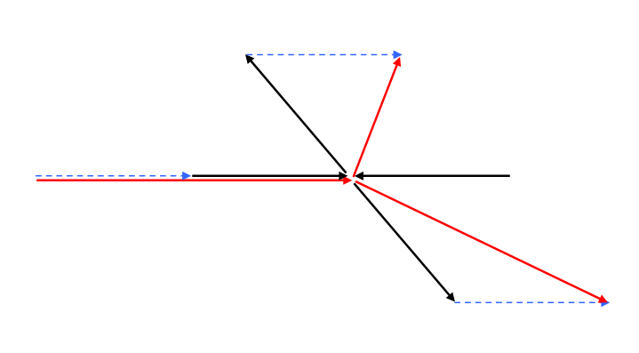
Note that for (nonrelativistic) equal mass particles, the scattering angle in the center of mass frame is twice the scattering angle in the fixed target (lab) frame. This is easily seen in the diagram below. The four equal-length black arrows, two in, two out, forming an X, are the center of mass momenta. The lab momenta are given by adding the (same length) blue dotted arrow to each, reducing one of the ingoing momenta to zero, and giving the (red arrow) lab momenta (slightly displaced for clarity). The outgoing lab momenta are the diagonals of rhombi (equal-side parallelograms), hence at right angles and bisecting the center of mass angles of scattering.