1.9: Radiances of Planetary Spheres

We conclude this chapter by applying some of the work covered so far to a planetary situation. We will consider two hypothetical planets idealised as smooth spheres. One planet will have a surface reflecting according to Lambert’s law, the other the Lommel-Seeliger law. The observer is able to resolve both planets equally well, so that we may compare and contrast the distribution of radiance across the projected discs at various phase angles.

Consider a unit sphere centred at the origin of an Oxyz coordinate system irradiated with flux density F from the x-direction. A distant observer in the xy plane detects the radiance at phase angle α (the angle Sun-planet-Earth). Using the spherical coordinates (1, Θ, Φ) for the surface of the sphere, it can be shown for the angles of incidence and reflection

\[\begin{array}{l}{\mu_{0}=\sin \Theta \cos \Phi} \\ {\mu=\sin \Theta \cos (\Phi-\alpha)}\end{array}\]

The projected sphere, the disc seen by the observer, will have projected coordinates

\[\begin{array}{l}{y^{\prime}=\sin \Theta \sin (\Phi-\alpha)} \\ {z=\cos \Theta}\end{array}\]

such that y'² + z² ≤ 1. Except at zero phase, not all the illuminated surface will be visible, since for each point on the disc both the condition μ₀ > 0 and μ > 0 must be satisfied in order that the point be both irradiated and not obscured from the observer.

Defining a quantity relative radiance, πL/ϖ₀F, we can directly compare the radiances of the two spheres, as shown in the table.

Relative Radiances of Spheres

Lambertian	μ0
Lommel-Seeliger	\(\frac{1}{4} \frac{\mu_{0}}{\mu_{0}+\mu}\)

The resulting images are readily programmed. In those that follow (le ftmost Lambertian, middle Lommel-Seeliger), each planet has been adjusted so that the maximum relative radiance is white. The rightmost image shows the outline of the lune visible to the observer.

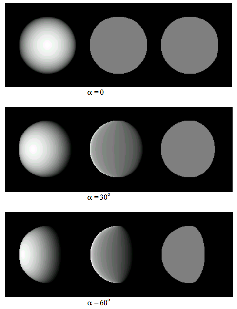
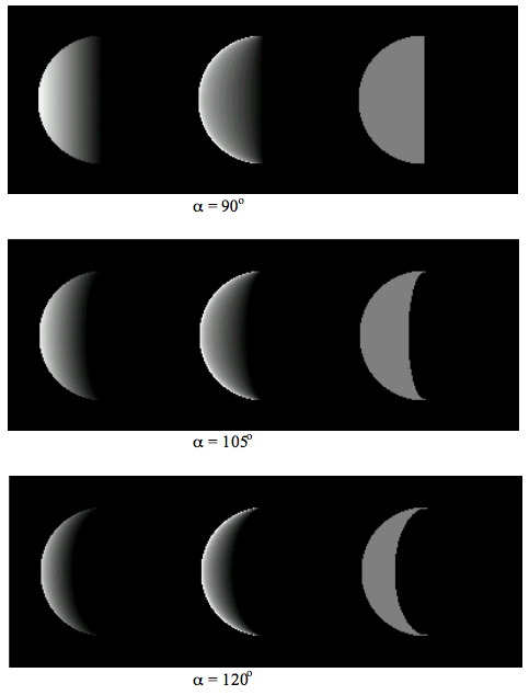
At opposition the Lambertian sphere is limb-darkened, whereas the Lommel-Seeliger sphere is uniformly bright. As the phase angle increases from zero the LommelSeeliger sphere becomes darkened towards the terminator and brightened at the limb. For phases greater than ninety degrees, the cusps of the Lommel-Seeliger sphere are more persistant than the Lambertian. Without commenting any further, the images do make interesting comparisons with the phases of the Moon.

Reference Notes.

Sections 2, 4, 5, 7, 8 and 9 are based on the author’s interpretation of Chandrasekhar’s book, chapters I, III, VI and IX.

1. Chandrasekhar, S., 1960, Radiative Transfer, Dover, New York.

The ideas of a quantity F defined only for a plane parallel beam and the use of the BRDF (bi-directional reflectance distribution function) for astronomical applications are taken from

2. Lester. P. L., McCall, M. L. & Tatum, J. B., 1979, J. Roy. Astron. Soc. Can., 73, 233

who use F for flux density, which clashes with the F of the πF used by Chandrasekhar – this is the reason for using F. (See also Nicodemus, F.E., Applied Optics, 4, 767 (1965) and 9, 1474 (1970) – JBT)

Section 10 is a revised and corrected adaptation of an article by the author

3. Fairbairn, M. B., 2002, J. Roy. Astron. Soc. Can., 96, 18.

Depending on the hardware used, the images shown may display some spurious contouring