
3: The Exponential Integral Function
- Page ID
- 6663

\( \newcommand{\vecs}[1]{\overset { \scriptstyle \rightharpoonup} {\mathbf{#1}} } \)
\( \newcommand{\vecd}[1]{\overset{-\!-\!\rightharpoonup}{\vphantom{a}\smash {#1}}} \)
\( \newcommand{\dsum}{\displaystyle\sum\limits} \)
\( \newcommand{\dint}{\displaystyle\int\limits} \)
\( \newcommand{\dlim}{\displaystyle\lim\limits} \)
\( \newcommand{\id}{\mathrm{id}}\) \( \newcommand{\Span}{\mathrm{span}}\)
( \newcommand{\kernel}{\mathrm{null}\,}\) \( \newcommand{\range}{\mathrm{range}\,}\)
\( \newcommand{\RealPart}{\mathrm{Re}}\) \( \newcommand{\ImaginaryPart}{\mathrm{Im}}\)
\( \newcommand{\Argument}{\mathrm{Arg}}\) \( \newcommand{\norm}[1]{\| #1 \|}\)
\( \newcommand{\inner}[2]{\langle #1, #2 \rangle}\)
\( \newcommand{\Span}{\mathrm{span}}\)
\( \newcommand{\id}{\mathrm{id}}\)
\( \newcommand{\Span}{\mathrm{span}}\)
\( \newcommand{\kernel}{\mathrm{null}\,}\)
\( \newcommand{\range}{\mathrm{range}\,}\)
\( \newcommand{\RealPart}{\mathrm{Re}}\)
\( \newcommand{\ImaginaryPart}{\mathrm{Im}}\)
\( \newcommand{\Argument}{\mathrm{Arg}}\)
\( \newcommand{\norm}[1]{\| #1 \|}\)
\( \newcommand{\inner}[2]{\langle #1, #2 \rangle}\)
\( \newcommand{\Span}{\mathrm{span}}\) \( \newcommand{\AA}{\unicode[.8,0]{x212B}}\)
\( \newcommand{\vectorA}[1]{\vec{#1}} % arrow\)
\( \newcommand{\vectorAt}[1]{\vec{\text{#1}}} % arrow\)
\( \newcommand{\vectorB}[1]{\overset { \scriptstyle \rightharpoonup} {\mathbf{#1}} } \)
\( \newcommand{\vectorC}[1]{\textbf{#1}} \)
\( \newcommand{\vectorD}[1]{\overrightarrow{#1}} \)
\( \newcommand{\vectorDt}[1]{\overrightarrow{\text{#1}}} \)
\( \newcommand{\vectE}[1]{\overset{-\!-\!\rightharpoonup}{\vphantom{a}\smash{\mathbf {#1}}}} \)
\( \newcommand{\vecs}[1]{\overset { \scriptstyle \rightharpoonup} {\mathbf{#1}} } \)
\(\newcommand{\longvect}{\overrightarrow}\)
\( \newcommand{\vecd}[1]{\overset{-\!-\!\rightharpoonup}{\vphantom{a}\smash {#1}}} \)
\(\newcommand{\avec}{\mathbf a}\) \(\newcommand{\bvec}{\mathbf b}\) \(\newcommand{\cvec}{\mathbf c}\) \(\newcommand{\dvec}{\mathbf d}\) \(\newcommand{\dtil}{\widetilde{\mathbf d}}\) \(\newcommand{\evec}{\mathbf e}\) \(\newcommand{\fvec}{\mathbf f}\) \(\newcommand{\nvec}{\mathbf n}\) \(\newcommand{\pvec}{\mathbf p}\) \(\newcommand{\qvec}{\mathbf q}\) \(\newcommand{\svec}{\mathbf s}\) \(\newcommand{\tvec}{\mathbf t}\) \(\newcommand{\uvec}{\mathbf u}\) \(\newcommand{\vvec}{\mathbf v}\) \(\newcommand{\wvec}{\mathbf w}\) \(\newcommand{\xvec}{\mathbf x}\) \(\newcommand{\yvec}{\mathbf y}\) \(\newcommand{\zvec}{\mathbf z}\) \(\newcommand{\rvec}{\mathbf r}\) \(\newcommand{\mvec}{\mathbf m}\) \(\newcommand{\zerovec}{\mathbf 0}\) \(\newcommand{\onevec}{\mathbf 1}\) \(\newcommand{\real}{\mathbb R}\) \(\newcommand{\twovec}[2]{\left[\begin{array}{r}#1 \\ #2 \end{array}\right]}\) \(\newcommand{\ctwovec}[2]{\left[\begin{array}{c}#1 \\ #2 \end{array}\right]}\) \(\newcommand{\threevec}[3]{\left[\begin{array}{r}#1 \\ #2 \\ #3 \end{array}\right]}\) \(\newcommand{\cthreevec}[3]{\left[\begin{array}{c}#1 \\ #2 \\ #3 \end{array}\right]}\) \(\newcommand{\fourvec}[4]{\left[\begin{array}{r}#1 \\ #2 \\ #3 \\ #4 \end{array}\right]}\) \(\newcommand{\cfourvec}[4]{\left[\begin{array}{c}#1 \\ #2 \\ #3 \\ #4 \end{array}\right]}\) \(\newcommand{\fivevec}[5]{\left[\begin{array}{r}#1 \\ #2 \\ #3 \\ #4 \\ #5 \\ \end{array}\right]}\) \(\newcommand{\cfivevec}[5]{\left[\begin{array}{c}#1 \\ #2 \\ #3 \\ #4 \\ #5 \\ \end{array}\right]}\) \(\newcommand{\mattwo}[4]{\left[\begin{array}{rr}#1 \amp #2 \\ #3 \amp #4 \\ \end{array}\right]}\) \(\newcommand{\laspan}[1]{\text{Span}\{#1\}}\) \(\newcommand{\bcal}{\cal B}\) \(\newcommand{\ccal}{\cal C}\) \(\newcommand{\scal}{\cal S}\) \(\newcommand{\wcal}{\cal W}\) \(\newcommand{\ecal}{\cal E}\) \(\newcommand{\coords}[2]{\left\{#1\right\}_{#2}}\) \(\newcommand{\gray}[1]{\color{gray}{#1}}\) \(\newcommand{\lgray}[1]{\color{lightgray}{#1}}\) \(\newcommand{\rank}{\operatorname{rank}}\) \(\newcommand{\row}{\text{Row}}\) \(\newcommand{\col}{\text{Col}}\) \(\renewcommand{\row}{\text{Row}}\) \(\newcommand{\nul}{\text{Nul}}\) \(\newcommand{\var}{\text{Var}}\) \(\newcommand{\corr}{\text{corr}}\) \(\newcommand{\len}[1]{\left|#1\right|}\) \(\newcommand{\bbar}{\overline{\bvec}}\) \(\newcommand{\bhat}{\widehat{\bvec}}\) \(\newcommand{\bperp}{\bvec^\perp}\) \(\newcommand{\xhat}{\widehat{\xvec}}\) \(\newcommand{\vhat}{\widehat{\vvec}}\) \(\newcommand{\uhat}{\widehat{\uvec}}\) \(\newcommand{\what}{\widehat{\wvec}}\) \(\newcommand{\Sighat}{\widehat{\Sigma}}\) \(\newcommand{\lt}{<}\) \(\newcommand{\gt}{>}\) \(\newcommand{\amp}{&}\) \(\definecolor{fillinmathshade}{gray}{0.9}\)Sooner or later (in particular in the next chapter) in the study of stellar atmospheres, we have need of the exponential integral function. This brief chapter contains nothing about stellar atmospheres or even astronomy, but it describes just as much as we need to know about the exponential integral function. It is not intended as a thorough exposition of everything that could be written about the function.
The exponential integral function of order \(n\), written as a function of a variable \(a\), is defined as
\[E_n(a) = \int_1^\infty x^{-n} e^{-ax} dx. \label{3.1} \]
I shall restrict myself to cases where \(n\) is a non-negative integer and \(a\) is a non-negative real variable. For stellar atmosphere theory in the next chapter we shall have need of \(n\) up to and including 3.
Let us start by seeing what the values of the functions are when \(a = 0\). We have
\[E_n (0) = \int_1^\infty x^{-n} dx \label{3.2} \]
and this is infinite for \(n = 0\) and for \(n = 1\). For larger \(n\) it is \(1/(n − 1)\).
Thus \(E_0(0) = \infty\), \(E_1 (0) = \infty\), \(E_2 (0) = 1\), \(E_3(0) = \frac{1}{2}\), \(E_4(0) = \frac{1}{3}\), etc.
Thereafter the functions (of whatever order) decrease monotonically as \(a\) increases, approaching zero asymptotically for large \(a\).
The function \(E_0(a)\) is easy to evaluate. It is
\[E_0(a) = \int_1^\infty e^{-ax} dx = \frac{e^{-a}}{a}. \label{3.3} \]
The evaluation of the exponential integral function for \(n > 0\) is less easy but it can be done by numerical (e.g. Simpson) integration. The upper limit of the integral in equation 3.1 is infinite, but this difficulty can be overcome by means of the substitution \(y = 1/x\), from which the equation becomes
\[E_n(0) = \int_0^1 y^{n-2} e^{-a/y} dy. \label{3.4} \]
Since both limits are finite, this can now in principle be integrated numerically in a straightforward way, for example by Simpson's rule or similar algorithm, except that, at the lower limit, \(a/y\) is infinite and it is necessary first to determine the limit of the integrand as \(y → 0\), which is zero.
There is, however, a way of evaluating the exponential integral function for \(n ≥ 2\) without the necessity of numerical integration. Consider, for example,
\[E_{n+1}(a) = \int_1^\infty x^{-(n+1)} e^{-ax} dx. \label{3.5} \]
If this is integrated (very carefully!) by parts, we arrive at
\[E_{n+1}(a) = \frac{1}{n} \left[ e^{-a} - aE_n (a) \right]. \label{3.6} \]
Thus from this recurrence relation, once we have evaluated \(E_1(a)\), we can evaluate \(E_2(a)\) and hence \(E_3(a)\) and so on.
The recurrence relation \(\ref{3.6}\), however, holds only for \(n ≥ 1\) (as will become apparent during the careful partial integration), so there is no getting around the numerical integration for \(n = 1\). Furthermore, for small values of \(a\) the functions for \(n = 0\) or \(1\) become very large, becoming infinite as \(a → 0\), which makes them very sensitive when trying to compute the next function up. Thus for small \(a\) or for constructing a table it may in the end be less trouble to take the bull by the horns and integrate them all numerically.
It will afford good programming practice to prepare a table of \(E_n(a)\) for \(a = 0\) to \(2\), in steps of \(0.01\), for \(n = 0, 1, 2, 3\). The table should ideally have five columns, the first being the \(201\) values of \(a\), and the remaining four being \(E_n(a)\), \(n = 1\) to \(4\). A graph of these functions is shown in figure \(\text{III.1}\).
In practice, in performing the calculations for figure \(\text{III.1}\), this is what I found. The function for \(n = 0\) was easy; it is given simply by equation \(\ref{3.3}\). For \(n = 1\), I integrated by Simpson's rule; \(100\) intervals in \(y\) was adequate to compute the function to nine decimal places. The function for \(n = 2\) was unexpectedly difficult. The recurrence relation \(\ref{3.6}\) was not useful at small \(a\), as discussed above. I therefore attempted to integrate it using Simpson's rule, yet, although the function is, on the face of it, very simple:
\[E_2(a) = \int_0^1 e^{-a/y} dy, \label{3.7} \]
Simpson's rule seemed inadequate to compute the function precisely even with as many as \(1000\) intervals in \(y\). Neither the recurrence relation nor numerical integration was without problems! I had no difficulty, however, with integrating the function with \(n = 3\), and so I then used the recurrence relation backwards to calculate the function for \(n = 2\) and all was well.
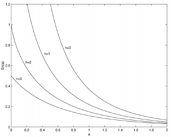
\(\text{FIGURE III.1}\)
The exponential integral function