
2: The Postulates of Quantum Mechanics
- Page ID
- 56456

\( \newcommand{\vecs}[1]{\overset { \scriptstyle \rightharpoonup} {\mathbf{#1}} } \)
\( \newcommand{\vecd}[1]{\overset{-\!-\!\rightharpoonup}{\vphantom{a}\smash {#1}}} \)
\( \newcommand{\dsum}{\displaystyle\sum\limits} \)
\( \newcommand{\dint}{\displaystyle\int\limits} \)
\( \newcommand{\dlim}{\displaystyle\lim\limits} \)
\( \newcommand{\id}{\mathrm{id}}\) \( \newcommand{\Span}{\mathrm{span}}\)
( \newcommand{\kernel}{\mathrm{null}\,}\) \( \newcommand{\range}{\mathrm{range}\,}\)
\( \newcommand{\RealPart}{\mathrm{Re}}\) \( \newcommand{\ImaginaryPart}{\mathrm{Im}}\)
\( \newcommand{\Argument}{\mathrm{Arg}}\) \( \newcommand{\norm}[1]{\| #1 \|}\)
\( \newcommand{\inner}[2]{\langle #1, #2 \rangle}\)
\( \newcommand{\Span}{\mathrm{span}}\)
\( \newcommand{\id}{\mathrm{id}}\)
\( \newcommand{\Span}{\mathrm{span}}\)
\( \newcommand{\kernel}{\mathrm{null}\,}\)
\( \newcommand{\range}{\mathrm{range}\,}\)
\( \newcommand{\RealPart}{\mathrm{Re}}\)
\( \newcommand{\ImaginaryPart}{\mathrm{Im}}\)
\( \newcommand{\Argument}{\mathrm{Arg}}\)
\( \newcommand{\norm}[1]{\| #1 \|}\)
\( \newcommand{\inner}[2]{\langle #1, #2 \rangle}\)
\( \newcommand{\Span}{\mathrm{span}}\) \( \newcommand{\AA}{\unicode[.8,0]{x212B}}\)
\( \newcommand{\vectorA}[1]{\vec{#1}} % arrow\)
\( \newcommand{\vectorAt}[1]{\vec{\text{#1}}} % arrow\)
\( \newcommand{\vectorB}[1]{\overset { \scriptstyle \rightharpoonup} {\mathbf{#1}} } \)
\( \newcommand{\vectorC}[1]{\textbf{#1}} \)
\( \newcommand{\vectorD}[1]{\overrightarrow{#1}} \)
\( \newcommand{\vectorDt}[1]{\overrightarrow{\text{#1}}} \)
\( \newcommand{\vectE}[1]{\overset{-\!-\!\rightharpoonup}{\vphantom{a}\smash{\mathbf {#1}}}} \)
\( \newcommand{\vecs}[1]{\overset { \scriptstyle \rightharpoonup} {\mathbf{#1}} } \)
\(\newcommand{\longvect}{\overrightarrow}\)
\( \newcommand{\vecd}[1]{\overset{-\!-\!\rightharpoonup}{\vphantom{a}\smash {#1}}} \)
\(\newcommand{\avec}{\mathbf a}\) \(\newcommand{\bvec}{\mathbf b}\) \(\newcommand{\cvec}{\mathbf c}\) \(\newcommand{\dvec}{\mathbf d}\) \(\newcommand{\dtil}{\widetilde{\mathbf d}}\) \(\newcommand{\evec}{\mathbf e}\) \(\newcommand{\fvec}{\mathbf f}\) \(\newcommand{\nvec}{\mathbf n}\) \(\newcommand{\pvec}{\mathbf p}\) \(\newcommand{\qvec}{\mathbf q}\) \(\newcommand{\svec}{\mathbf s}\) \(\newcommand{\tvec}{\mathbf t}\) \(\newcommand{\uvec}{\mathbf u}\) \(\newcommand{\vvec}{\mathbf v}\) \(\newcommand{\wvec}{\mathbf w}\) \(\newcommand{\xvec}{\mathbf x}\) \(\newcommand{\yvec}{\mathbf y}\) \(\newcommand{\zvec}{\mathbf z}\) \(\newcommand{\rvec}{\mathbf r}\) \(\newcommand{\mvec}{\mathbf m}\) \(\newcommand{\zerovec}{\mathbf 0}\) \(\newcommand{\onevec}{\mathbf 1}\) \(\newcommand{\real}{\mathbb R}\) \(\newcommand{\twovec}[2]{\left[\begin{array}{r}#1 \\ #2 \end{array}\right]}\) \(\newcommand{\ctwovec}[2]{\left[\begin{array}{c}#1 \\ #2 \end{array}\right]}\) \(\newcommand{\threevec}[3]{\left[\begin{array}{r}#1 \\ #2 \\ #3 \end{array}\right]}\) \(\newcommand{\cthreevec}[3]{\left[\begin{array}{c}#1 \\ #2 \\ #3 \end{array}\right]}\) \(\newcommand{\fourvec}[4]{\left[\begin{array}{r}#1 \\ #2 \\ #3 \\ #4 \end{array}\right]}\) \(\newcommand{\cfourvec}[4]{\left[\begin{array}{c}#1 \\ #2 \\ #3 \\ #4 \end{array}\right]}\) \(\newcommand{\fivevec}[5]{\left[\begin{array}{r}#1 \\ #2 \\ #3 \\ #4 \\ #5 \\ \end{array}\right]}\) \(\newcommand{\cfivevec}[5]{\left[\begin{array}{c}#1 \\ #2 \\ #3 \\ #4 \\ #5 \\ \end{array}\right]}\) \(\newcommand{\mattwo}[4]{\left[\begin{array}{rr}#1 \amp #2 \\ #3 \amp #4 \\ \end{array}\right]}\) \(\newcommand{\laspan}[1]{\text{Span}\{#1\}}\) \(\newcommand{\bcal}{\cal B}\) \(\newcommand{\ccal}{\cal C}\) \(\newcommand{\scal}{\cal S}\) \(\newcommand{\wcal}{\cal W}\) \(\newcommand{\ecal}{\cal E}\) \(\newcommand{\coords}[2]{\left\{#1\right\}_{#2}}\) \(\newcommand{\gray}[1]{\color{gray}{#1}}\) \(\newcommand{\lgray}[1]{\color{lightgray}{#1}}\) \(\newcommand{\rank}{\operatorname{rank}}\) \(\newcommand{\row}{\text{Row}}\) \(\newcommand{\col}{\text{Col}}\) \(\renewcommand{\row}{\text{Row}}\) \(\newcommand{\nul}{\text{Nul}}\) \(\newcommand{\var}{\text{Var}}\) \(\newcommand{\corr}{\text{corr}}\) \(\newcommand{\len}[1]{\left|#1\right|}\) \(\newcommand{\bbar}{\overline{\bvec}}\) \(\newcommand{\bhat}{\widehat{\bvec}}\) \(\newcommand{\bperp}{\bvec^\perp}\) \(\newcommand{\xhat}{\widehat{\xvec}}\) \(\newcommand{\vhat}{\widehat{\vvec}}\) \(\newcommand{\uhat}{\widehat{\uvec}}\) \(\newcommand{\what}{\widehat{\wvec}}\) \(\newcommand{\Sighat}{\widehat{\Sigma}}\) \(\newcommand{\lt}{<}\) \(\newcommand{\gt}{>}\) \(\newcommand{\amp}{&}\) \(\definecolor{fillinmathshade}{gray}{0.9}\)The entire structure of quantum mechanics (including its relativistic extension) can be formulated in terms of states and operations in Hilbert space. We need rules that map the physical quantities such as states, observables, and measurements to the mathematical structure of vector spaces, vectors and operators. There are several ways in which this can be done, and here we summarize these rules in terms of five postulates.
A physical system is described by a Hilbert space \(\mathscr{H}\), and the state of the system is represented by a ray with norm 1 in \(\mathscr{H}\).
There are a number of important aspects to this postulate. First, the fact that states are rays, rather than vectors means that an overall phase \(e^{i \varphi}\) of the state does not have any physically observable consequences, and \(e^{i \varphi}|\psi\rangle\) represents the same state as \(|\psi\rangle\). Second, the state contains all information about the system. In particular, there are no hidden variables in this standard formulation of quantum mechanics. Finally, the dimension of \(\mathscr{H}\) may be infinite, which is the case, for example, when \(\mathscr{H}\) is the space of square-integrable functions.
As an example of this postulate, consider a two-level quantum system (a qubit). This system can be described by two orthonormal states \(|0\rangle\) and \(|1\rangle\). Due to linearity of Hilbert space, the superposition \(\alpha|0\rangle+\beta|1\rangle\) is again a state of the system if it has norm 1, or
\[(\alpha ^ { * } \langle0|+\beta^{*}\langle 1|)(\alpha|0\rangle+\beta|1\rangle)=1 \quad \text { or } \quad|\alpha|^{2}+|\beta|^{2}=1\tag{2.1}\]
This is called the superposition principle: any normalised superposition of valid quantum states is again a valid quantum state. It is a direct consequence of the linearity of the vector space, and as we shall see later, this principle has some bizarre consequences that have been corroborated in many experiments.
Every physical observable \(A\) corresponds to a self-adjoint (Hermitian1) operator \(\hat{A}\) whose eigenvectors form a complete basis.
We use a hat to distinguish between the observable and the operator, but usually this distinction is not necessary. In these notes, we will use hats only when there is a danger of confusion.
As an example, take the operator \(X\):
\[X|0\rangle=|1\rangle \quad \text { and } \quad X|1\rangle=|0\rangle.\tag{2.2}\]
This operator can be interpreted as a bit flip of a qubit. In matrix notation the state vectors can be written as
\[|0\rangle=\left(\begin{array}{l}1 \\ 0 \end{array}\right) \quad \text { and } \quad|1\rangle=\left(\begin{array}{l} 0 \\ 1 \end{array}\right),\tag{2.3}\]
which means that \(X\) is written as
\[X=\left(\begin{array}{ll}
0 & 1 \\
1 & 0
\end{array}\right)\tag{2.4}\]
with eigenvalues ±1. The eigenstates of \(X\) are
\[|\pm\rangle=\frac{|0\rangle \pm|1\rangle}{\sqrt{2}}.\tag{2.5}\]
These states form an orthonormal basis.
The eigenvalues of \(A\) are the possible measurement outcomes, and the probability of finding the outcome \(a_{j}\) in a measurement is given by the Born rule:
\[p\left(a_{j}\right)=\left|\left\langle a_{j} \mid \psi\right\rangle\right|^{2},\tag{2.6}\]
where \(|\psi\rangle\) is the state of the system, and \(\left|a_{j}\right\rangle\) is the eigenvector associated with the eigenvalue \(a_{j}\) via \(A\left|a_{j}\right\rangle=a_{j}\left|a_{j}\right\rangle\). If \(a_{j}\) is \(m\)-fold degenerate, then
\[p(a_{j})=\sum_{l=1}^{m}|\langle a_{j}^{(l)} \mid \psi\rangle|^{2},\tag{2.7}\]
where the \(\left|a_{j}^{(l)}\right\rangle\) span the \(m\)-fold degenerate subspace
The expectation value of \(A\) with respect to the state of the system \(|\psi\rangle\) is denoted by \(\langle A\rangle\), and evaluated as
\[\langle A\rangle=\langle\psi|A| \psi\rangle=\langle\psi|(\sum_{j} a_{j}|a_{j}\rangle\langle a_{j}|)| \psi\rangle=\sum_{j} p(a_{j}) a_{j}\tag{2.8}\]
This is the weighted average of the measurement outcomes. The spread of the measurement outcomes (or the uncertainty) is given by the variance
\[(\Delta A)^{2}=\left\langle(A-\langle A\rangle)^{2}\right\rangle=\left\langle A^{2}\right\rangle-\langle A\rangle^{2}\tag{2.9}\]
So far we mainly dealt with discrete systems on finite-dimensional Hilbert spaces. But what about continuous systems, such as a particle in a box, or a harmonic oscillator? We can still write the spectral decomposition of an operator A but the sum must be replace by an integral:
\[A=\int d a f_{A}(a)|a\rangle\langle a|\tag{2.10}\]
where \(|a\rangle\) is an eigenstate of \(A\). Typically, there are problems with the normalization of \(|a\rangle\), which is related to the impossibility of preparing a system in exactly the state \(|a\rangle\). We will not explore these subtleties further in this course, but you should be aware that they exist. The expectation value of \(A\) is
\[\langle A\rangle=\langle\psi|A| \psi\rangle=\int d a f_{A}(a)\langle\psi \mid a\rangle\langle a \mid \psi\rangle \equiv \int d a f_{A}(a)|\psi(a)|^{2},\tag{2.11}\]
where we defined the wave function \(\psi(a)=\langle a \mid \psi\rangle\), and \(|\psi(a)|^{2}\) is properly interpreted as the probability density that you remember from second-year quantum mechanics.
The probability of finding the eigenvalue of an operator \(A\) in the interval \(a\) and \(a+d a\) given the state \(|\psi\rangle\) is
\[\langle\psi|(|a\rangle\langle a| d a)| \psi\rangle \equiv d p(a),\tag{2.12}\]
since both sides must be infinitesimal. We therefore find that
\[\frac{d p(a)}{d a}=|\psi(a)|^{2}\tag{2.13}\]
The dynamics of quantum systems is governed by unitary transformations
We can write the state of a system at time \(t\) as \(|\psi(t)\rangle\), and at some time \(t_{0}<t\) as \(\left|\psi\left(t_{0}\right)\right\rangle\). The fourth postulate tells us that there is a unitary operator \(U\left(t, t_{0}\right)\) that transforms the state at time \(t_{0}\) to the state at time \(t\):
\[|\psi(t)\rangle=U\left(t, t_{0}\right)\left|\psi\left(t_{0}\right)\right\rangle\tag{2.14}\]
Since the evolution from time \(t\) to \(t\) is denoted by \(U(t, t)\) and must be equal to the identity, we deduce that \(U\) depends only on time differences: \(U\left(t, t_{0}\right)=U\left(t-t_{0}\right)\), and \(U(0)=\mathbb{I}\).
As an example, let \(U(t)\) be generated by a Hermitian operator \(A\) according to
\(U(t)=\exp \left(-\frac{i}{\hbar} A t\right)\tag{2.15}\)
The argument of the exponential must be dimensionless, so \(A\) must be proportional to \(\hbar\) times an angular frequency (in other words, an energy). Suppose that \(|\psi(t)\rangle\) is the state of a qubit, and that \(A=\hbar \omega X\). If \(|\psi(0)\rangle=|0\rangle\) we want to calculate the state of the system at time \(t\). We can write
\[|\psi(t)\rangle=U(t)|\psi(0)\rangle=\exp (-i \omega t X)|0\rangle=\sum_{n=0}^{\infty} \frac{(-i \omega t)^{n}}{n !} X^{n}\tag{2.16}\]
Observe that \(X^{2}=\mathbb{I}\), so we can separate the power series into even and odd values of n:
\[|\psi(t)\rangle=\sum_{n=0}^{\infty} \frac{(-i \omega t)^{2 n}}{(2 n) !}|0\rangle+\sum_{n=0}^{\infty} \frac{(-i \omega t)^{2 n+1}}{(2 n+1) !} X|0\rangle=\cos (\omega t)|0\rangle-i \sin (\omega t)|1\rangle\tag{2.17}\]
In other words, the state oscillates between \(|0\rangle\) and \(|1\rangle\).
The fourth postulate also leads to the Schrödinger equation. Let’s take the infinitesimal form of Eq. (2.14):
\[|\psi(t+d t)\rangle=U(d t)|\psi(t)\rangle\tag{2.18}\]
We require that \(U(d t)\) is generated by some Hermitian operator \(H\):
\[U(d t)=\exp \left(-\frac{i}{\hbar} H d t\right)\tag{2.19}\]
\(H\) must have the dimensions of energy, so we identify it with the energy operator, or the Hamiltonian. We can now take a Taylor expansion of \(|\psi(t+d t)\rangle\) to first order in dt:
\[|\psi(t+d t)\rangle=|\psi(t)\rangle+d t \frac{d}{d t}|\psi(t)\rangle+\ldots,\tag{2.20}\]
and we expand the unitary operator to first order in dt as well:
\[U(d t)=1-\frac{i}{\hbar} H d t+\ldots\tag{2.21}\]
We combine this into
\[|\psi(t)\rangle+d t \frac{d}{d t}|\psi(t)\rangle=\left(1-\frac{i}{\hbar} H d t\right)|\psi(t)\rangle,\tag{2.22}\]
which can be recast into the Schrödinger equation:
\[i \hbar \frac{d}{d t}|\psi(t)\rangle=H|\psi(t)\rangle\tag{2.23}\]Therefore, the Schrödinger equation follows directly from the postulates!
If a measurement of an observable \(A\) yields an eigenvalue \(a_{j}\), then immediately after the measurement, the system is in the eigenstate \(\left|a_{j}\right\rangle\) corresponding to the eigenvalue
This is the infamous projection postulate, so named because a measurement “projects” the system to the eigenstate corresponding to the measured value. This postulate has as observable consequence that a second measurement immediately after the first will also find the outcome \(a_{j}\). Each measurement outcome \(a_{j}\) corresponds to a projection operator \(P_{j}\) on the subspace spanned by the eigenvector(s) belonging to \(a_{j}\). A (perfect) measurement can be described by applying a projector to the state, and renormalize:
\[|\psi\rangle \rightarrow \frac{P_{j}|\psi\rangle}{\| P_{j}|\psi\rangle \|}\tag{2.24}\]
This also works for degenerate eigenvalues.
We have established earlier that the expectation value of \(A\) can be written as a trace:
\[\langle A\rangle=\operatorname{Tr}(|\psi\rangle\langle\psi| A)\tag{2.25}\]
Now instead of the full operator \(A\), we calculate the trace of \(P_{j}=\left|a_{j}\right\rangle\left\langle a_{j}\right|\):
\[\left\langle P_{j}\right\rangle=\operatorname{Tr}\left(|\psi\rangle\langle\psi| P_{j}\right)=\operatorname{Tr}\left(|\psi\rangle\left\langle\psi \mid a_{j}\right\rangle\left\langle a_{j}\right|\right)=\left|\left\langle a_{j} \mid \psi\right\rangle\right|^{2}=p\left(a_{j}\right)\tag{2.26}\]
So we can calculate the probability of a measurement outcome by taking the expectation value of the projection operator that corresponds to the eigenstate of the measurement outcome. This is one of the basic calculations in quantum mechanics that you should be able to do.
The Measurement Problem
The projection postulate is somewhat problematic for the interpretation of quantum mechanics, because it leads to the so-called measurement problem: Why does a measurement induce a non-unitary evolution of the system? After all, the measurement apparatus can also be described quantum mechanically2 and then the system plus the measurement apparatus evolves unitarily. But then we must invoke a new device that measures the combined system and measurement apparatus. However, this in turn can be described quantum mechanically, and so on.
On the other hand, we do see definite measurement outcomes when we do experiments, so at some level the projection postulate is necessary, and somewhere there must be a “collapse of the wave function”. Schrödinger already struggled with this question, and came up with his famous thought experiment about a cat in a box with a poison-filled vial attached to a Geiger counter monitoring a radioactive atom (Figure 1). When the atom decays, it will trigger the Geiger counter, which in turn causes the release of the poison killing the cat. When we do not look inside the box (more precisely: when no information about the atom-counter-vial-cat system escapes from the box), the entire system is in a quantum superposition. However, when we open the box, we do find the cat either dead or alive. One solution of the problem seems to be that the quantum state represents our knowledge of the system, and that looking inside the box merely updates our information about the atom, counter, vial and the cat. So nothing “collapses” except our own state of mind.
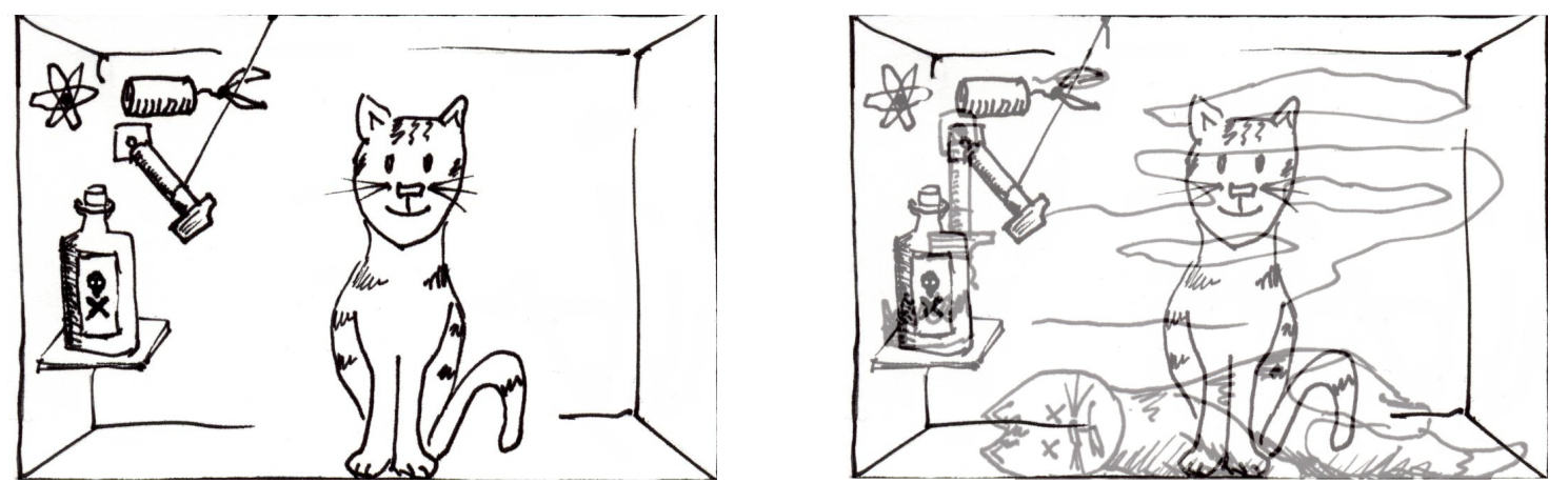 Figure 1: Schrödingers Cat.
However, this cannot be the entire story, because quantum mechanics clearly is not just about our opinions of cats and decaying atoms. In particular, if we prepare an electron in a spin “up” state \(|\uparrow\rangle\), then whenever we measure the spin along the \(z\)-direction we will find the measurement outcome “up”, no matter what we think about electrons and quantum mechanics. So there seems to be some physical property associated with the electron that determines the measurement outcome and is described by the quantum state.
Various interpretations of quantum mechanics attempt to address these (and other) issues. The original interpretation of quantum mechanics was mainly put forward by Niels Bohr, and is called the Copenhagen interpretation. Broadly speaking, it says that the quantum state is a convenient fiction, used to calculate the results of measurement outcomes, and that the system cannot be considered separate from the measurement apparatus. Alternatively, there are interpretations of quantum mechanics, such as the Ghirardi-Rimini-Weber interpretation, that do ascribe some kind of reality to the state of the system, in which case a physical mechanism for the collapse of the wave function must be given. Many of these interpretations can be classified as hidden variable theories, which postulate that there is a deeper physical reality described by some “hidden variables” that we must average over. This in turn explains the probabilistic nature of quantum mechanics. The problem with such theories is that these hidden variables must be quite weird: they can change instantly depending on events light-years away3 , thus violating Einstein’s theory of special relativity. Many physicists do not like this aspect of hidden variable theories.
Alternatively, quantum mechanics can be interpreted in terms of “many worlds”: the Many Worlds interpretation states that there is one state vector for the entire universe, and that each measurement splits the universe into different branches corresponding to the different measurement outcomes. It is attractive since it seems to be a philosophically consistent interpretation, and while it has been acquiring a growing number of supporters over recent years4, a lot of physicists have a deep aversion to the idea of parallel universes.
Finally, there is the epistemic interpretation, which is very similar to the Copenhagen interpretation in that it treats the quantum state to a large extent as a measure of our knowledge of the quantum system (and the measurement apparatus). At the same time, it denies a deeper underlying reality (i.e., no hidden variables). The attractive feature of this interpretation is that it requires a minimal amount of fuss, and fits naturally with current research in quantum information theory. The downside is that you have to abandon simple scientific realism that allows you to talk about the properties of electrons and photons, and many physicists are not prepared to do that.
As you can see, quantum mechanics forces us to abandon some deeply held (classical) convictions about Nature. Depending on your preference, you may be drawn to one or other interpretation. It is currently not know which interpretation is the correct one.
- Calculate the eigenvalues and the eigenstates of the bit flip operator \(X\), and show that the eigenstates form an orthonormal basis. Calculate the expectation value of \(X\) for \(|\psi\rangle=1 / \sqrt{3}|0\rangle+i \sqrt{2 / 3}|1\rangle\).
- Show that the variance of \(A\) vanishes when \(|\psi\rangle\) is an eigenstate of \(A\).
- Prove that an operator is Hermitian if and only if it has real eigenvalues.
- Show that a qubit in an unknown state \(|\psi\rangle\) cannot be copied. This is the no-cloning theorem. Hint: start with a state \(|\psi\rangle|i\rangle\) for some initial state \(|i\rangle\), and require that for \(|\psi\rangle=|0\rangle\) and \(|\psi\rangle=|1\rangle\) the cloning procedure is a unitary transformation \(|0\rangle|i\rangle \rightarrow|0\rangle|0\rangle\) and \(|1\rangle|i\rangle \rightarrow|1\rangle|1\rangle\).
- The uncertainty principle.
- Use the Cauchy-Schwarz inequality to derive the following relation between non-commuting observables \(A\) and \(B\):
\[(\Delta A)^{2}(\Delta B)^{2} \geq \frac{1}{4}|\langle[A, B]\rangle|^{2}\tag{2.27}\]
Hint: define \(|f\rangle=(A-\langle A\rangle)|\psi\rangle\) and \(|g\rangle=i(B-\langle B\rangle)|\psi\rangle\), and use that \(|\langle f \mid g\rangle| \geq \frac{1}{2} \mid\langle f \mid g\rangle+\langle g|f\rangle|\).
- Show that this reduces to Heisenberg’s uncertainty relation when \(A\) and \(B\) are canonically conjugate observables, for example position and momentum.
- Does this method work for deriving the uncertainty principle between energy and time?
- Use the Cauchy-Schwarz inequality to derive the following relation between non-commuting observables \(A\) and \(B\):
- Consider the Hamiltonian \(H\) and the state \(|\psi\rangle\) given by
\[H=E\left(\begin{array}{ccc}
0 & i & 0 \\
-i & 0 & 0 \\
0 & 0 & -1
\end{array}\right) \quad \text { and } \quad|\psi\rangle=\frac{1}{\sqrt{5}}\left(\begin{array}{c}
1-i \\
1-i \\
1
\end{array}\right)\tag{2.28}\]where \(E\) is a constant with dimensions of energy. Calculate the energy eigenvalues and the expectation value of the Hamiltonian.
- Show that the momentum and the total energy can be measured simultaneously only when the potential is constant everywhere. What does a constant potential mean in terms of the dynamics of a particle?
1In Hilbert spaces of infinite dimensionality, there are subtle differences between self-adjoint and Hermitian operators. We ignore these subtleties here, because we will be mostly dealing with finite-dimensional spaces.
2This is something most people require from a fundamental theory: quantum mechanics should not just break down for macroscopic objects. Indeed, experimental evidence of macroscopic superpositions has been found in the form of “cat states”.
3 . . . even though the averaging over the hidden variables means you can never signal faster than light.
4There seems to be some evidence that the Many Worlds interpretation fits well with the latest cosmological models based on string theory