
8.7: Energy-Shifts and Decay-Widths

( \newcommand{\kernel}{\mathrm{null}\,}\)
We have examined how a state |n⟩ , other than the initial state |i⟩ , becomes populated as a result of some time-dependent perturbation applied to the system. Let us now consider how the initial state becomes depopulated.
In this case, it is convenient to gradually turn on the perturbation from zero at t=−∞ . Thus,
H1(t)=exp(ηt)H1, ???where η is small and positive, and H1 is a constant.
In the remote past, t→−∞ , the system is assumed to be in the initial state |i⟩ . Thus, ci(t→−∞)=1 , and cn≠i(t→−∞)=0 . Basically, we want to calculate the time evolution of the coefficient ci(t) . First, however, let us check that our previous Fermi golden rule result still applies when the perturbing potential is turned on slowly, instead of very suddenly. For cn≠i(t) we have from Equations ???-??? that
c???n(t) =0, ??? c???n(t)![$ = - \frac{\rm i}{\hbar}\, H_{ni} \int_{-\infty}^t dt'\, \exp[(\et...
..., \frac{ \exp[(\eta + {\rm i}\,\omega_{ni} )\, t]}{\eta +{\rm i}\,\omega_{ni}},$](http://farside.ph.utexas.edu/teaching/qm/lectures/img1950.png) ???
??? where Hni=⟨n|H1|i⟩ . It follows that, to first order, the transition probability from state |i⟩ to state |n⟩ is
Pi→n(t)=|c???n|2=|Hni|2ℏ2exp(2ηt)η2+ω2ni. ???The transition rate is given by
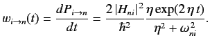 ???
??? Consider the limit η→0 . In this limit, exp(ηt)→1 , but
limη→0ηη2+ω 2ni=πδ(ωni)=πℏδ(En−Ei). ???Thus, Equation ??? yields the standard Fermi golden rule result
wi→n=2πℏ|Hni|2δ(En−Ei). ???It is clear that the delta-function in the above formula actually represents a function that is highly peaked at some particular energy. The width of the peak is determined by how fast the perturbation is switched on.
Let us now calculate ci(t) using Equations ???-???. We have
c???i(t) =1, ??? c???i(t) =−iℏHii∫t−∞exp(ηt′)dt′=−iℏHiiexp(ηt)η, ??? c???i(t)![$ = \left(\frac{-{\rm i}}{\hbar} \right)^2 \sum_m \vert H_{mi}\vert...
...xp[(\eta+ {\rm i}\,\omega_{im})\, t'] \exp[ (\eta+ {\rm i}\,\omega_{mi})\, t'']$](http://farside.ph.utexas.edu/teaching/qm/lectures/img1962.png) =(−iℏ)2∑m|Hmi|2exp(2ηt)2η(η+iωmi). ???
=(−iℏ)2∑m|Hmi|2exp(2ηt)2η(η+iωmi). ??? Thus, to second order we have
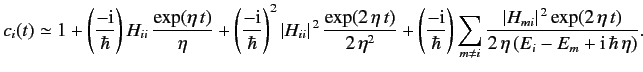 ???
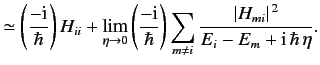
??? Let us now consider the ratio ˙ci/ci , where ![]() . Using Equation ???, we can evaluate this ratio in the limit η→0 . We obtain
. Using Equation ???, we can evaluate this ratio in the limit η→0 . We obtain
![$ \simeq \left[\left( \frac{-{\rm i}}{\hbar}\right) H_{ii} + \left(...
...a}\right]\left/\left( 1- \frac{\rm i}{\hbar} \frac{H_{ii}}{\eta} \right)\right.$](http://farside.ph.utexas.edu/teaching/qm/lectures/img1968.png)
 ???
??? This result is formally correct to second order in perturbed quantities. Note that the right-hand side of Equation ??? is independent of time. We can write
˙cici=(−iℏ)Δi, ???where
Δi=Hii+limη→0∑m≠i|Hmi|2Ei−Em+iℏη ???is a constant. According to a well-known result in pure mathematics,
limϵ→01x+iϵ=P1x−iπδ(x), ???where ϵ>0 , and P denotes the principal part. It follows that
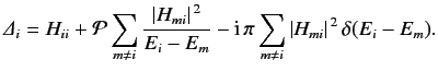 ???
??? It is convenient to normalize the solution of Equation ??? such that ci???=1 . Thus, we obtain
ci(t)=exp(−iΔitℏ). ???According to Equation ???, the time evolution of the initial state ket |i⟩ is given by
|i,t⟩=exp[−i(Δi+Ei)t/ℏ]|i⟩. ???We can rewrite this result as
|i,t⟩=exp(−i[Ei+Re(Δi)]t/ℏ)exp[Im(Δi)t/ℏ]|i⟩. ???It is clear that the real part of Δi gives rise to a simple shift in energy of state |i⟩ , whereas the imaginary part of Δi governs the growth or decay of this state. Thus,
|i,t⟩=exp[−i(Ei+ΔEi)t/ℏ]exp(−Γit/2ℏ)|i⟩, ???where
ΔEi=Re(Δi)=Hii+P∑m≠i|Hmi|2Ei−Em, ???and
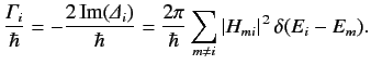 ???
??? Note that the energy-shift ΔEi is the same as that predicted by standard time-independent perturbation theory.
The probability of observing the system in state |i⟩ at time t>0 , given that it is definately in state |i⟩ at time t=0 , is given by
Pi→i(t)=|ci|2=exp(−Γit/ℏ), ???where
Γiℏ=∑m≠iwi→m. ???Here, use has been made of Equation ???. Clearly, the rate of decay of the initial state is a simple function of the transition rates to the other states. Note that the system conserves probability up to second order in perturbed quantities, because
|ci|2+∑m≠i|cm|2≃(1−Γit/ℏ)+∑m≠iwi→mt=1. ???The quantity Γi is called the decay-width of state |i⟩ . It is closely related to the mean lifetime of this state,
τi=ℏΓi, ???where
Pi→i=exp(−t/τi). ???According to Equation ???, the amplitude of state |i⟩ both oscillates and decays as time progresses. Clearly, state |i⟩ is not a stationary state in the presence of the time-dependent perturbation. However, we can still represent it as a superposition of stationary states (whose amplitudes simply oscillate in time). Thus,
exp[−i(Ei+ΔEi)t/ℏ]exp(−Γit/2ℏ)=∫dEf(E)exp(−iEt/ℏ), ???where f(E) is the weight of the stationary state with energy E in the superposition. The Fourier inversion theorem yields
|f(E)|2∝1(E−[Ei+Re(Δi)])2+Γ2i/4. ???In the absence of the perturbation, |f(E)|2 is basically a delta-function centered on the unperturbed energy Ei of state |i⟩ . In other words, state |i⟩ is a stationary state whose energy is completely determined. In the presence of the perturbation, the energy of state |i⟩ is shifted by Re(Δi) . The fact that the state is no longer stationary (i.e., it decays in time) implies that its energy cannot be exactly determined. Indeed, the energy of the state is smeared over some region of width (in energy) Γi centered around the shifted energy Ei+Re(Δi) . The faster the decay of the state (i.e., the larger Γi ), the more its energy is spread out. This effect is clearly a manifestation of the energy-time uncertainty relation ΔEΔt∼ℏ . One consequence of this effect is the existence of a natural width of spectral lines associated with the decay of some excited state to the ground state (or any other lower energy state). The uncertainty in energy of the excited state, due to its propensity to decay, gives rise to a slight smearing (in wavelength) of the spectral line associated with the transition. Strong lines, which correspond to fast transitions, are smeared out more that weak lines. For this reason, spectroscopists generally favor forbidden lines (see Section 8.10) for Doppler-shift measurements. Such lines are not as bright as those corresponding to allowed transitions, but they are a lot sharper.
Contributors
Richard Fitzpatrick (Professor of Physics, The University of Texas at Austin)