11.5i: Light damping- \( \gamma < 2\omega_{0}\)
- Page ID
- 8954

Since \( \gamma < 2\omega_{0}\), we have to write Equations 11.5.6 as
\[ k_{1}=-\frac{1}{2}\gamma+i\sqrt{\omega_{0}^{2}-\frac{1}{4}\gamma^{2}},\quad k_{2}=-\frac{1}{2}\gamma-i\sqrt{\omega_{0}^{2}-\frac{1}{4}\gamma^{2}}. \label{11.5.7}\tag{11.5.7} \]
Further, I shall write
\[ \omega^{'}=\sqrt{w_{0}^{2}-\frac{1}{4}\gamma^{2}}. \label{11.5.8}\tag{11.5.8} \]
Equation 11.5.4 is therefore
\[ x=Ae^{-\frac{1}{2}\gamma t+i\omega^{'}t}+Be^{-\frac{1}{2}\gamma t-i\omega^{'}t}=e^{-\frac{1}{2}\gamma t}(Ae^{+i\omega^{'}t}+Be^{-i\omega^{'}t}). \tag{11.5.9}\label{11.5.9} \]
If \( x\) is to be real, \( A\) and \( B\) must be complex. Also, since \( e^{-i\omega^{'}t}=(e^{i\omega^{'}t})\)* must equal \( A\)*, where the asterisk denotes the complex conjugate.
Let \( A=\frac{1}{2}(a-ib)\) and \( B=\frac{1}{2}(a+ib)\) where \( a\) and \( b\) are real. Then the reader should be able to show that Equation \( \ref{11.5.9}\) can be written as
\[ x=e^{-\frac{1}{2}\gamma t}(a\cos\omega^{'}t+b\sin\omega^{'}t). \label{11.5.10}\tag{11.5.10} \]
And if \( C=\sqrt{a^{2}+b^{2}}, \sin\alpha=\frac{a}{\sqrt{a^{2}+b^{2}}}, \cos\alpha=\frac{b}{\sqrt{a^{2}+b^{2}}},\) the equation can be written
\[ x=Ce^{-\frac{1}{2}\gamma t}\sin(\omega^{'}t+\alpha). \label{11.5.11}\tag{11.5.11} \]
Equations \( \ref{11.5.9}\), \( \ref{11.5.10}\) or \( \ref{11.5.11}\) are three equivalent ways of writing the solution. Each has two arbitrary integration constants \( (A,B), (a,b)\) or \( (C,\alpha)\), whose values depend on the initial conditions - i.e. on the values of \( x\) and \( \dot{x}\) when \( t=0\). Equation \( \ref{11.5.11}\) shows that the motion is a sinusoidal oscillation of period a little less than \( \omega_{0}\), with an exponentially decreasing amplitude.
To find \( C\) and \( \alpha\) in terms of the initial conditions, differentiate Equation \( \ref{11.5.11}\) with respect to the time in order to obtain an equation showing the speed as a function of the time:
\[ \dot{x}=Ce^{-\frac{1}{2}\gamma t}[\omega^{'}\cos(\omega^{'}t+\alpha)-\frac{1}{2}\gamma\sin(\omega^{'}t+\alpha)]. \label{11.5.12}\tag{11.5.12} \]
By putting \( t=0\) in Equations \( \ref{11.5.11}\) and \( \ref{11.5.12}\) we obtain
\[ x_{0}=C\sin\alpha \label{11.5.13}\tag{11.5.13} \]
and
\[ (\dot{x})_{0}=C(\omega^{'}\cos\alpha-\frac{1}{2}\gamma\sin\alpha). \label{11.5.14}\tag{11.5.14} \]
From these we easily obtain
\[ \cot\alpha=\frac{1}{\omega^{'}}[\frac{(\dot{x})_{0}}{\dot{x}_{0}}+\frac{\gamma}{2}] \label{11.5.15}\tag{11.5.15} \]
and
\[ C=x_{0}\csc\alpha. \label{11.5.16}\tag{11.5.16} \]
The quadrant of \( \alpha\) can be determined from the signs of \( \cot\alpha\) and \( \csc\alpha\) , \( C\) always being positive.
Note that the amplitude of the motion falls off with time as \( e^{-\frac{1}{2}\gamma t}\), but the mechanical energy, which is proportional to the square of the amplitude, falls off as \( e^{-\gamma t}\).
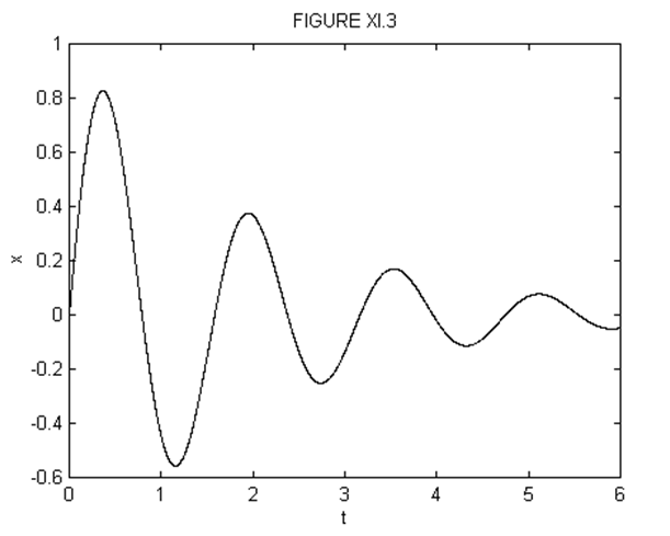
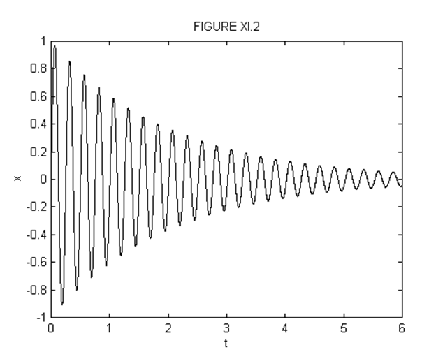
Figures XI.2 and XI.3 are drawn for \( C=1, \alpha=0, \gamma=1\). Figure XI.2 has \( \omega_{0}=25\gamma\) and hence \( x=e^{-\frac{1}{2}t}\sin0.24.9949995t\), and figure XI.3 has \( \omega_{0}=4\gamma\) and hence \( x=e^{-\frac{1}{2}t}\sin3.968626967t\).
Draw displacement : time graphs for an oscillator with \( m\) = 0.02 kg, \( k\) = 0.08 N m-1, \( g\) = 1.5 s-1, \( t\) = 0 to 15 s, for the following initial conditions:
- \( x_{0}=0,\quad (\dot{x})_{0}=4\) ms-1
- \( (\dot{x})_{0}=0,\quad x_{0}=3\) m
- \( (\dot{x})=-2\) ms-1, \(x_{0}=2\)
Although the motion of a damped oscillator is not strictly "periodic", in that the motion does not repeat itself exactly, we could define a "period" \( P=\frac{2\pi}{\omega^{'}}\) as the interval between two consecutive ascending zeroes. Extrema do not occur exactly halfway between consecutive zeroes, and the reader should have no difficulty in showing, by differentiation of Equation \( \ref{11.5.11}\), that extrema occur at times given by \( \tan(\omega^{'}t+\alpha)=\frac{2\omega^{'}}{\gamma}\). However, provided that the damping is not very large, consecutive extrema occur approximately at intervals of \( \frac{P}{2}\). The ratio of consecutive maximum displacements is, then,
\[ \frac{|x_{n}|}{|x_{n+1}|}=\frac{e^{-\frac{1}{2}\gamma t}}{e^{-\frac{1}{2}\gamma (t+\frac{1}{2}P)}}. \label{11.5.17}\tag{11.5.17} \]
From this, we find that the logarithmic decrement is
\[ ln(\frac{|x_{n}|}{|x_{n+1}|})=\frac{P\gamma}{4}, \label{11.5.18}\tag{11.5.18} \]
from which the damping constant can be determined.