
11.4: Worked Examples
- Page ID
- 24490
\( \newcommand{\vecs}[1]{\overset { \scriptstyle \rightharpoonup} {\mathbf{#1}} } \)
\( \newcommand{\vecd}[1]{\overset{-\!-\!\rightharpoonup}{\vphantom{a}\smash {#1}}} \)
\( \newcommand{\dsum}{\displaystyle\sum\limits} \)
\( \newcommand{\dint}{\displaystyle\int\limits} \)
\( \newcommand{\dlim}{\displaystyle\lim\limits} \)
\( \newcommand{\id}{\mathrm{id}}\) \( \newcommand{\Span}{\mathrm{span}}\)
( \newcommand{\kernel}{\mathrm{null}\,}\) \( \newcommand{\range}{\mathrm{range}\,}\)
\( \newcommand{\RealPart}{\mathrm{Re}}\) \( \newcommand{\ImaginaryPart}{\mathrm{Im}}\)
\( \newcommand{\Argument}{\mathrm{Arg}}\) \( \newcommand{\norm}[1]{\| #1 \|}\)
\( \newcommand{\inner}[2]{\langle #1, #2 \rangle}\)
\( \newcommand{\Span}{\mathrm{span}}\)
\( \newcommand{\id}{\mathrm{id}}\)
\( \newcommand{\Span}{\mathrm{span}}\)
\( \newcommand{\kernel}{\mathrm{null}\,}\)
\( \newcommand{\range}{\mathrm{range}\,}\)
\( \newcommand{\RealPart}{\mathrm{Re}}\)
\( \newcommand{\ImaginaryPart}{\mathrm{Im}}\)
\( \newcommand{\Argument}{\mathrm{Arg}}\)
\( \newcommand{\norm}[1]{\| #1 \|}\)
\( \newcommand{\inner}[2]{\langle #1, #2 \rangle}\)
\( \newcommand{\Span}{\mathrm{span}}\) \( \newcommand{\AA}{\unicode[.8,0]{x212B}}\)
\( \newcommand{\vectorA}[1]{\vec{#1}} % arrow\)
\( \newcommand{\vectorAt}[1]{\vec{\text{#1}}} % arrow\)
\( \newcommand{\vectorB}[1]{\overset { \scriptstyle \rightharpoonup} {\mathbf{#1}} } \)
\( \newcommand{\vectorC}[1]{\textbf{#1}} \)
\( \newcommand{\vectorD}[1]{\overrightarrow{#1}} \)
\( \newcommand{\vectorDt}[1]{\overrightarrow{\text{#1}}} \)
\( \newcommand{\vectE}[1]{\overset{-\!-\!\rightharpoonup}{\vphantom{a}\smash{\mathbf {#1}}}} \)
\( \newcommand{\vecs}[1]{\overset { \scriptstyle \rightharpoonup} {\mathbf{#1}} } \)
\(\newcommand{\longvect}{\overrightarrow}\)
\( \newcommand{\vecd}[1]{\overset{-\!-\!\rightharpoonup}{\vphantom{a}\smash {#1}}} \)
\(\newcommand{\avec}{\mathbf a}\) \(\newcommand{\bvec}{\mathbf b}\) \(\newcommand{\cvec}{\mathbf c}\) \(\newcommand{\dvec}{\mathbf d}\) \(\newcommand{\dtil}{\widetilde{\mathbf d}}\) \(\newcommand{\evec}{\mathbf e}\) \(\newcommand{\fvec}{\mathbf f}\) \(\newcommand{\nvec}{\mathbf n}\) \(\newcommand{\pvec}{\mathbf p}\) \(\newcommand{\qvec}{\mathbf q}\) \(\newcommand{\svec}{\mathbf s}\) \(\newcommand{\tvec}{\mathbf t}\) \(\newcommand{\uvec}{\mathbf u}\) \(\newcommand{\vvec}{\mathbf v}\) \(\newcommand{\wvec}{\mathbf w}\) \(\newcommand{\xvec}{\mathbf x}\) \(\newcommand{\yvec}{\mathbf y}\) \(\newcommand{\zvec}{\mathbf z}\) \(\newcommand{\rvec}{\mathbf r}\) \(\newcommand{\mvec}{\mathbf m}\) \(\newcommand{\zerovec}{\mathbf 0}\) \(\newcommand{\onevec}{\mathbf 1}\) \(\newcommand{\real}{\mathbb R}\) \(\newcommand{\twovec}[2]{\left[\begin{array}{r}#1 \\ #2 \end{array}\right]}\) \(\newcommand{\ctwovec}[2]{\left[\begin{array}{c}#1 \\ #2 \end{array}\right]}\) \(\newcommand{\threevec}[3]{\left[\begin{array}{r}#1 \\ #2 \\ #3 \end{array}\right]}\) \(\newcommand{\cthreevec}[3]{\left[\begin{array}{c}#1 \\ #2 \\ #3 \end{array}\right]}\) \(\newcommand{\fourvec}[4]{\left[\begin{array}{r}#1 \\ #2 \\ #3 \\ #4 \end{array}\right]}\) \(\newcommand{\cfourvec}[4]{\left[\begin{array}{c}#1 \\ #2 \\ #3 \\ #4 \end{array}\right]}\) \(\newcommand{\fivevec}[5]{\left[\begin{array}{r}#1 \\ #2 \\ #3 \\ #4 \\ #5 \\ \end{array}\right]}\) \(\newcommand{\cfivevec}[5]{\left[\begin{array}{c}#1 \\ #2 \\ #3 \\ #4 \\ #5 \\ \end{array}\right]}\) \(\newcommand{\mattwo}[4]{\left[\begin{array}{rr}#1 \amp #2 \\ #3 \amp #4 \\ \end{array}\right]}\) \(\newcommand{\laspan}[1]{\text{Span}\{#1\}}\) \(\newcommand{\bcal}{\cal B}\) \(\newcommand{\ccal}{\cal C}\) \(\newcommand{\scal}{\cal S}\) \(\newcommand{\wcal}{\cal W}\) \(\newcommand{\ecal}{\cal E}\) \(\newcommand{\coords}[2]{\left\{#1\right\}_{#2}}\) \(\newcommand{\gray}[1]{\color{gray}{#1}}\) \(\newcommand{\lgray}[1]{\color{lightgray}{#1}}\) \(\newcommand{\rank}{\operatorname{rank}}\) \(\newcommand{\row}{\text{Row}}\) \(\newcommand{\col}{\text{Col}}\) \(\renewcommand{\row}{\text{Row}}\) \(\newcommand{\nul}{\text{Nul}}\) \(\newcommand{\var}{\text{Var}}\) \(\newcommand{\corr}{\text{corr}}\) \(\newcommand{\len}[1]{\left|#1\right|}\) \(\newcommand{\bbar}{\overline{\bvec}}\) \(\newcommand{\bhat}{\widehat{\bvec}}\) \(\newcommand{\bperp}{\bvec^\perp}\) \(\newcommand{\xhat}{\widehat{\xvec}}\) \(\newcommand{\vhat}{\widehat{\vvec}}\) \(\newcommand{\uhat}{\widehat{\uvec}}\) \(\newcommand{\what}{\widehat{\wvec}}\) \(\newcommand{\Sighat}{\widehat{\Sigma}}\) \(\newcommand{\lt}{<}\) \(\newcommand{\gt}{>}\) \(\newcommand{\amp}{&}\) \(\definecolor{fillinmathshade}{gray}{0.9}\)Example 11.1 Relative Velocities of Two Moving Planes
An airplane A is traveling northeast with a speed of \(v_{\mathrm{A}}=160 \mathrm{m} \cdot \mathrm{s}^{-1}\). A second airplane B is traveling southeast with a speed of \(v_{\mathrm{B}}=200 \mathrm{m} \cdot \mathrm{s}^{-1}\). (a) Choose a coordinate system and write down an expression for the velocity of each airplane as vectors, \(\overrightarrow{\mathbf{V}}_{\mathrm{A}}\) and \(\overrightarrow{\mathbf{V}}_{B}\) Carefully use unit vectors to express your answer. (b) Sketch the vectors \(\overrightarrow{\mathbf{V}}_{\mathbf{A}}\) and \(\overrightarrow{\mathbf{V}}_{\mathbf{B}}\) on your coordinate system. (c) Find a vector expression that expresses the velocity of aircraft A as seen from an observer flying in aircraft B. Calculate this vector. What is its magnitude and direction? Sketch it on your coordinate system.
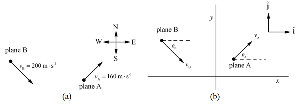
An observer at rest with respect to the ground defines a reference frame \(S\). Choose a coordinate system shown in Figure 11.2b. According to this observer, airplane A is moving with velocity \(\overrightarrow{\mathbf{v}}_{\mathrm{A}}=v_{\mathrm{A}} \cos \theta_{\mathrm{A}} \hat{\mathbf{i}}+v_{\mathrm{A}} \sin \theta_{\mathrm{A}} \hat{\mathbf{j}}\), and airplane B is moving with velocity \(\overrightarrow{\mathbf{v}}_{\mathrm{B}}=v_{\mathrm{B}} \cos \theta_{\mathrm{B}} \hat{\mathbf{i}}+v_{\mathrm{B}} \sin \theta_{\mathrm{B}} \hat{\mathbf{j}}\). According to the information given in the problem airplane A flies northeast so \(\theta_{\mathrm{A}}=\pi / 4\) and airplane B flies southeast east so \(\theta_{\mathrm{B}}=-\pi / 4\). Thus \(\overrightarrow{\mathbf{v}}_{\mathrm{A}}=\left(80 \sqrt{2} \mathrm{m} \cdot \mathrm{s}^{-1}\right) \hat{\mathbf{i}}+\left(80 \sqrt{2} \mathrm{m} \cdot \mathrm{s}^{-1}\right) \hat{\mathbf{j}}\) and \(\overrightarrow{\mathbf{v}}_{\mathrm{B}}=\left(100 \sqrt{2} \mathrm{m} \cdot \mathrm{s}^{-1}\right) \hat{\mathbf{i}}-\left(100 \sqrt{2} \mathrm{m} \cdot \mathrm{s}^{-1}\right) \hat{\mathbf{j}}\).
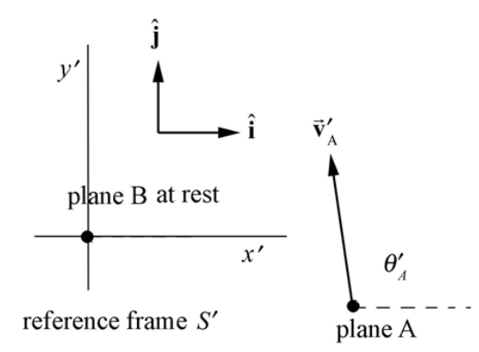
Consider a second observer moving along with airplane B, defining reference frame S′ . What is the velocity of airplane A according to this observer moving in airplane B ? The velocity of the observer moving along in airplane B with respect to an observer at rest on the ground is just the velocity of airplane B and is given by \(\overrightarrow{\mathbf{V}}=\overrightarrow{\mathbf{v}}_{\mathrm{B}}=v_{\mathrm{B}} \cos \theta_{\mathrm{B}} \hat{\mathbf{i}}+v_{\mathrm{B}} \sin \theta_{\mathrm{B}} \hat{\mathbf{j}}\). Using the Law of Addition of Velocities, Equation (11.3.2), the velocity of airplane A with respect to an observer moving along with Airplane B is given by
\[\begin{aligned}
\overrightarrow{\mathbf{v}}_{\mathrm{A}}^{\prime} &=\overrightarrow{\mathbf{v}}_{\mathrm{A}}-\overrightarrow{\mathbf{V}}=\left(v_{\mathrm{A}} \cos \theta_{\mathrm{A}} \hat{\mathbf{i}}+v_{\mathrm{A}} \sin \theta_{\mathrm{A}} \hat{\mathbf{j}}\right)-\left(v_{\mathrm{B}} \cos \theta_{\mathrm{B}} \hat{\mathbf{i}}+v_{\mathrm{B}} \sin \theta_{\mathrm{B}} \hat{\mathbf{j}}\right) \\
&=\left(v_{\mathrm{A}} \cos \theta_{\mathrm{A}}-v_{\mathrm{B}} \cos \theta_{\mathrm{B}}\right) \hat{\mathbf{i}}+\left(v_{\mathrm{A}} \sin \theta_{\mathrm{A}}-v_{\mathrm{B}} \sin \theta_{\mathrm{B}}\right) \hat{\mathbf{j}} \\
&=\left(\left(80 \sqrt{2} \mathrm{m} \cdot \mathrm{s}^{-1}\right)-\left(100 \sqrt{2} \mathrm{m} \cdot \mathrm{s}^{-1}\right)\right) \hat{\mathbf{i}}+\left(\left(80 \sqrt{2} \mathrm{m} \cdot \mathrm{s}^{-1}\right)+\left(100 \sqrt{2} \mathrm{m} \cdot \mathrm{s}^{-1}\right)\right) \hat{\mathbf{j}} . \\
&=-\left(20 \sqrt{2} \mathrm{m} \cdot \mathrm{s}^{-1}\right) \hat{\mathbf{i}}+\left(180 \sqrt{2} \mathrm{m} \cdot \mathrm{s}^{-1}\right) \hat{\mathbf{j}} \\
&=v_{A x}^{\prime} \hat{\mathbf{i}}+v_{A \mathrm{y}}^{\prime} \hat{\mathbf{j}}
\end{aligned} \nonumber \]
Figure 11.3 shows the velocity of airplane A with respect to airplane B in reference frame S′ .
The magnitude of velocity of airplane A as seen by an observer moving with airplane B is given by
\[\left|\vec{v}_{\mathrm{A}}^{\prime}\right|=\left(v_{A x}^{\prime 2}+v_{A y}^{\prime 2}\right)^{1 / 2}=\left(\left(-20 \sqrt{2} \mathrm{m} \cdot \mathrm{s}^{-1}\right)^{2}+\left(180 \sqrt{2} \mathrm{m} \cdot \mathrm{s}^{-1}\right)^{2}\right)^{1 / 2}=256 \mathrm{m} \cdot \mathrm{s}^{-1} \nonumber \]
The angle of velocity of airplane A as seen by an observer moving with airplane B is given by,
\[\begin{aligned}
\theta_{A}^{\prime} &=\tan ^{-1}\left(v_{A y}^{\prime} / v_{A x}^{\prime}\right)=\tan ^{-1}\left(\left(180 \sqrt{2} \mathrm{m} \cdot \mathrm{s}^{-1}\right) /\left(-20 \sqrt{2} \mathrm{m} \cdot \mathrm{s}^{-1}\right)\right) \\
&=\tan ^{-1}(-9)=180^{\circ}-83.7^{\circ}=96.3^{\circ}
\end{aligned} \nonumber \]
Example 11.2 Relative Motion and Polar Coordinates
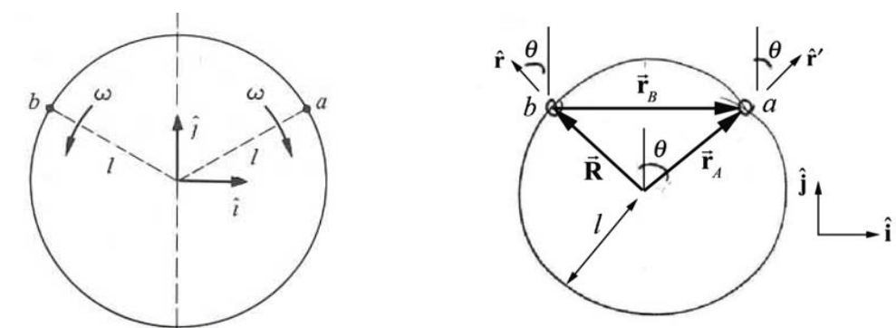
By relative velocity we mean velocity with respect to a specified coordinate system. (The term velocity, alone, is understood to be relative to the observer’s coordinate system.) (a) A point is observed to have velocity \(\overrightarrow{\mathbf{V}}_{A}\), relative to coordinate system A . What is its velocity relative to coordinate system B , which is displaced from system A by distance \(\overrightarrow{\mathbf{R}}\)? \((\overrightarrow{\mathbf{R}}\) can change in time.) (b) Particles a and b move in opposite directions around a circle with the magnitude of the angular velocity ω , as shown in Figure 11.4. At t = 0 they are both at the point \(\overrightarrow{\mathbf{r}}=\hat{l} \hat{\mathbf{j}}\) where l is the radius of the circle. Find the velocity of a relative to b .
Solution: (a) The position vectors are related by
\[\overrightarrow{\mathbf{r}}_{B}=\overrightarrow{\mathbf{r}}_{A}-\overrightarrow{\mathbf{R}} \nonumber \]
The velocities are related by the taking derivatives, (law of addition of velocities Equation (11.3.2))
\[\overrightarrow{\mathbf{v}}_{B}=\overrightarrow{\mathbf{v}}_{A}-\overrightarrow{\mathbf{V}} \nonumber \]
(b) Let’s choose two reference frames; frame B is centered at particle b, and frame A is centered at the center of the circle in Figure 11.5. Then the relative position vector between the origins of the two frames is given by
\[\overrightarrow{\mathbf{R}}=l \hat{\mathbf{r}} \nonumber \]
The position vector of particle a relative to frame A is given by
\[\overrightarrow{\mathbf{r}}_{A}=l \hat{\mathbf{r}}^{\prime} \nonumber \]
The position vector of particle b in frame B can be found by substituting Equations (11.4.7) and (11.4.6) into Equation (11.4.4),
\[\overrightarrow{\mathbf{r}}_{B}=\overrightarrow{\mathbf{r}}_{A}-\overrightarrow{\mathbf{R}}=l \hat{\mathbf{r}}^{\prime}-l \hat{\mathbf{r}} \nonumber \]
We can decompose each of the unit vectors \(\hat{\mathbf{r}}\) and \(\hat{\mathbf{r}}^{\prime}\) with respect to the Cartesian unit vectors \(\hat{\mathbf{1}}\) and \(\hat{\mathbf{j}}\) (see Figure 11.5),
\[\hat{\mathbf{r}}=-\sin \theta \hat{\mathbf{i}}+\cos \theta \hat{\mathbf{j}} \nonumber \]
\[\hat{\mathbf{r}}^{\prime}=\sin \theta \hat{\mathbf{i}}+\cos \theta \hat{\mathbf{j}} \nonumber \]
Then Equation (11.4.8) giving the position vector of particle b in frame B becomes
\[\overrightarrow{\mathbf{r}}_{B}=l \hat{\mathbf{r}}^{\prime}-l \hat{\mathbf{r}}=l(\sin \theta \hat{\mathbf{i}}+\cos \theta \hat{\mathbf{j}})-l(-\sin \theta \hat{\mathbf{i}}+\cos \theta \hat{\mathbf{j}})=2 l \sin \theta \hat{\mathbf{i}} \nonumber \]
In order to find the velocity vector of particle a in frame B (i.e. with respect to particle b), differentiate Equation (11.4.11)
\[\overrightarrow{\mathbf{v}}_{B}=\frac{d}{d t}(2 l \sin \theta) \hat{\mathbf{i}}=(2 l \cos \theta) \frac{d \theta}{d t} \hat{\mathbf{i}}=2 \omega l \cos \theta \hat{\mathbf{i}} \nonumber \]
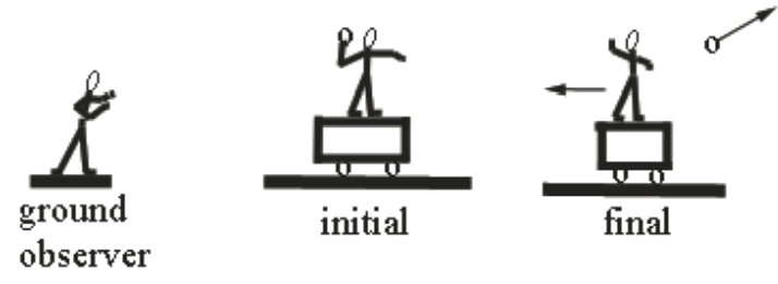
Example 11.3 Recoil in Different Frames
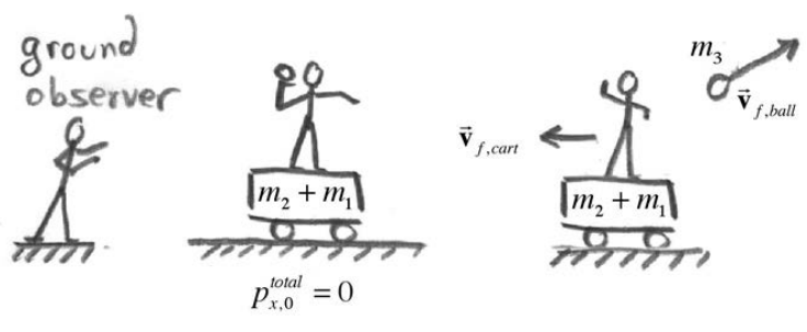
A person of mass \(m_{1}\) is standing on a cart of mass \(m_{2}\). Assume that the cart is free to move on its wheels without friction. The person throws a ball of mass \(m_{3}\) θ with respect to the horizontal as measured by the person in the cart. The ball is thrown with a speed \(v_{0}\) with respect to the cart (Figure 11.6). (a) What is the final velocity of the ball as seen by an observer fixed to the ground? (b) What is the final velocity of the cart as seen by an observer fixed to the ground? (c) With respect to the horizontal, what angle the fixed observer see the ball leave the cart?
Solution: a), b) Our reference frame will be that fixed to the ground. We shall take as our initial state that before the ball is thrown (cart, ball, throwing person stationary) and our final state that after the ball is thrown. We are assuming that there is no friction, and so there are no external forces acting in the horizontal direction. The initial x -component of the total momentum is zero,
\(p_{x, 0}=0\) total
After the ball is thrown, the cart and person have a final momentum
\[\overrightarrow{\mathbf{p}}_{f, \text { cart }}=-\left(m_{2}+m_{1}\right) v_{f, \text { cart }} \hat{\mathbf{i}} \nonumber \]
as measured by the person on the ground, where \(v_{f, cart}=0\) is the speed of the person and cart. (The person’s center of mass will move with respect to the cart while the ball is being thrown, but since we’re interested in velocities, not positions, we need only assume that the person is at rest with respect to the cart after the ball is thrown.)
The ball is thrown with a speed \(v_{0}\) and at an angle θ with respect to the horizontal as measured by the person in the cart. Therefore the person in the cart throws the ball with velocity
\[\overrightarrow{\mathbf{v}}_{f, \text { ball }}^{\prime}=v_{0} \cos \theta \hat{\mathbf{i}}+v_{0} \sin \theta \hat{\mathbf{j}} \nonumber \]
Because the cart is moving in the negative x -direction with speed \(v_{f, cart}=0\) just as the ball leaves the person’s hand, the x -component of the velocity of the ball as measured by an observer on the ground is given by
\[v_{x f, \text { ball }}=v_{0} \cos \theta-v_{f, \text { cart }} \nonumber \]
The ball appears to have a smaller x -component of the velocity according to the observer on the ground. The velocity of the ball as measured by an observer on the ground is
\[\overrightarrow{\mathbf{v}}_{f, \text { ball }}=\left(v_{0} \cos \theta-v_{f, \text { cart }}\right) \hat{\mathbf{i}}+v_{0} \sin \theta \hat{\mathbf{j}} \nonumber \]
The final momentum of the ball according to an observer on the ground is
\[\overrightarrow{\mathbf{p}}_{f, \text { ball }}=m_{3}\left[\left(v_{0} \cos \theta-v_{f, \text { can }}\right) \hat{\mathbf{i}}+v_{0} \sin \theta \hat{\mathbf{j}}\right] \nonumber \]
The momentum flow diagram is shown in (Figure 11.7).
Because the x -component of the momentum of the system is constant, we have that
\[\begin{aligned}
0 &=\left(p_{x, f}\right)_{\text {cart }}+\left(p_{x, f}\right)_{\text {ball }} \\
&=-\left(m_{2}+m_{1}\right) v_{f, \text { cart }}+m_{3}\left(v_{0} \cos \theta-v_{f, \text { cart }}\right)
\end{aligned} \nonumber \]
We can solve Equation (11.4.19) for the final speed and velocity of the cart as measured by an observer on the ground,
\[v_{f, \text { cart }}=\frac{m_{3} v_{0} \cos \theta}{m_{2}+m_{1}+m_{3}} \nonumber \]
\[\overrightarrow{\mathbf{v}}_{f, \text { cart }}=v_{f, \text { cart }} \hat{\mathbf{i}}=\frac{m_{3} v_{0} \cos \theta}{m_{2}+m_{1}+m_{3}} \hat{\mathbf{i}} \nonumber \]
Note that the y -component of the momentum is not constant because as the person is throwing the ball he or she is pushing off the cart and the normal force with the ground exceeds the gravitational force so the net external force in the y -direction is non-zero.
Substituting Equation (11.4.20) into Equation (11.4.17) gives
\[\begin{aligned}
\overrightarrow{\mathbf{v}}_{f, \text { ball }} &=\left(v_{0} \cos \theta-v_{f, \text { cart }}\right) \hat{\mathbf{i}}+v_{0} \sin \theta \hat{\mathbf{j}} \\
&=\frac{m_{1}+m_{2}}{m_{1}+m_{2}+m_{3}}\left(v_{0} \cos \theta\right) \hat{\mathbf{i}}+\left(v_{0} \sin \theta\right) \hat{\mathbf{j}}
\end{aligned} \nonumber \]
As a check, note that in the limit \(m_{3}<<m_{1}+m_{2}\), \(\overrightarrow{\mathbf{V}} f, \text { ball }\) has speed \(v_{0}\) and is directed at an angle θ above the horizontal; the fact that the much more massive person-cart combination is free to move doesn’t affect the flight of the ball as seen by the fixed observer. Also note that in the unrealistic limit \(m>>m_{1}+m_{2}\) the ball is moving at a speed much smaller than \(v_{0}\) as it leaves the cart.
c) The angle \(\phi\) at which the ball is thrown as seen by the observer on the ground is given by
\[\begin{aligned}
\phi &=\tan ^{-1} \frac{\left(v_{f, \text { ball }}\right)_{y}}{\left(v_{f, \text { ball }}\right)_{x}}=\tan ^{-1} \frac{v_{0} \sin \theta}{\left[\left(m_{1}+m_{2}\right) /\left(m_{1}+m_{2}+m_{3}\right)\right] v_{0} \cos \theta} \\
&=\tan ^{-1}\left[\left(\frac{m_{1}+m_{2}+m_{3}}{m_{1}+m_{2}}\right) \tan \theta\right]
\end{aligned} \nonumber \]
For arbitrary values for the masses, the above expression will not reduce to a simplified form. However, we can see that \(\tan \phi>\tan \theta\) for arbitrary masses, and that in the limit \(m_{3}<<m_{1}+m_{2}, \phi \rightarrow \theta\) and in the unrealistic limit \(m_{3} \gg m_{1}+m_{2}, \phi \rightarrow \pi / 2\). Can you explain this last odd prediction?