1.3: The Bernoulli Effect

Suppose air is being pumped down a smooth round tube, which has a constant diameter except for a section in the middle where the tube narrows down to half the diameter, then widens out again. Assume all the changes in diameter take place smoothly, and the air flows steadily down the tube, with no eddies or turbulence.

Exercise

where in the tube do you expect the pressure to be greatest?

Answer

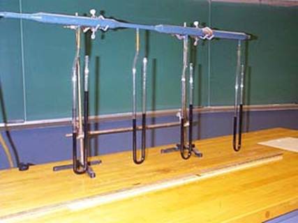
Most people asked this for the first time predict that the pressure will be greatest in the narrow portion of the tube. But in fact, if we actually do the experiment, by putting pressure gauges at various points along the tube, we find, counter intuitively, that the air pressure is lowest where the air is moving fastest!

Figure \(\PageIndex{1}\): The difference in heights of the dark liquid in the two arms of the U-tubes measures the pressure difference between that point in the flow tube and the outside atmospheric pressure.

To see how this could be, we will apply the techniques we developed to find how pressure varied in a stationary fluid. The way we did that, remember, was by drawing a free body diagram for a small cylinder of fluid. Since this small cylinder was at rest, the total force on it was zero, so the net pressure balanced the weight. Now consider a steadily moving fluid. It’s helpful to visualize the flow by drawing in streamlines, lines such that their direction is the direction the fluid is moving in at each point.

Actually, these streamlines not only tell you the direction the fluid is moving in, but also gives some idea of the speed—where they come closer together, the fluid must be moving faster, because the same amount of fluid is flowing through a narrower region. Imagine now a cylinder of air moving along the pipe, its axis parallel to the streamline. Obviously, it must speed up as it enters the narrow part of the tube—since the same amount of air is flowing through the narrow part as the wide part, it must be going faster.

But if the small cylinder of fluid is accelerating, it must be acted on by a force pushing it from behind.

Its weight is irrelevant here, since it’s moving horizontally. Therefore the only force acting on it is the pressure, and we have to conclude that the pressure at its back is greater than the pressure on its front. Therefore the pressure must be dropping on entering the narrow part. To make clearer what’s going on, we’ll draw a rather large cylinder:

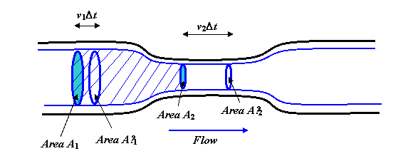
The fluid is flowing steadily and smoothly along the pipe. The thick blue lines are streamlines, in fact you should imagine rotating the whole diagram about the central axis to get a three-dimensional picture, and the blue lines would become a cylinder, with a narrower “neck” section, echoing the shape of the pipe.

Now consider the body of fluid within the streamlines shown, and capped at the two ends by the circular areas A₁ and A₂. The rate of flow of fluid across A₁ must be the same as the rate of flow across A₂, because in steady flow fluid can’t be piling up in the middle (or depleting from there either). The volume flowing across A₁ in one second is v₁A₁. (To see this, imagine a long straight pipe without a narrow part. If the fluid is flowing at, say 3 meters per second, then in one second all the fluid which was within 3 meters of the area A₁ on the upstream side will have flowed through.)

So, flow across A₁ equals flow across A₂, \[ A_1v_1 = A_2v_2 .\]

(Footnote: It’s perhaps worth mentioning that we are implicitly assuming the velocity is the same at all points on area A₁. Any real fluid has some viscosity (friction) and will be moving more slowly near the sides of the pipe than in the middle. We’ll discuss this later. For now, we consider an “ideal” fluid, the term used when one ignores viscosity. In fact, the result we derive is ok—we could have taken a tiny area A₁ far away from the sides, so that the velocity would have been the same for the whole area, but that would have given a much less clear diagram.)

We’re now ready to examine the increase in kinetic energy of the fluid as it speeds up into the narrow part, and understand how the pressure difference did the work necessary to speed it up.

Suppose that after a time Dt, the fluid that was at an initial instant between A₁ and A₂ has moved to the volume between A′₁ and A′₂. As far as the chunk of fluid we’re tracking is concerned, it has effectively replaced a volume \( A_1v_1 \Delta t \) moving at v₁ with a volume \( A_2v_2 \Delta t \) moving at v₂. But remember \( A_1v_1 = A_2v_2 \), so if the density of the fluid is \( \rho \) , we’re talking about a mass of fluid \( \rho A_1v_1 \Delta t \) which has effectively increased in speed from v₁ to v₂. That is to say, the increase in kinetic energy is just

\[ \Delta(K.E.) = \dfrac {1}{2}(\rho A_1v_1 \Delta t)(v_2^2 - v_1^2) .\]

The only possible source for this increase in energy is the work done by pressure in pushing the fluid into the narrow part.

Taking the pressure on area A₁ to be P₁, the total force on A₁ is \( P_1A_1 \). In the time\( \Delta t \), this force acts through a distance \( v_1 \Delta t \), and hence does

\[ work = force \times distance = P_1A_1v_1 \Delta t .\]

So this is work done on our chunk of fluid by the fluid pushing it from behind—but that’s not the end of the story, because our chunk of fluid itself does work pushing the fluid in front of it, so to find the total increase in our chunk’s energy, we must subtract off the external work it does. That is, the total work done by pressure on our fluid is

\[ P_1A_1v_1 \Delta t - P_2A_2v_2 \Delta t = (P_1 - P_2) A_1v_1 \Delta t \]

remembering that \( A_1v_1 = A_2v_2 \).

This work done must equal the change in kinetic energy, so

\[ (P_1 - P_2)A_1v_1 \Delta t = \dfrac {1}{2} ( \rho A_1v_1 \Delta t)(V_2^2 - v_1^2) \]

from which

\[ P_1 + \dfrac {1}{2} \rho v_1^2 = P_2 + \dfrac{1}{2} \rho v_2^2 \]

This is Bernoulli’s equation.

There is a further easy generalization: we could have the pipe sloping uphill. In that case, the fluid would gain potential energy as well as kinetic energy, so the pressure would have to do more work. If we take the center of the area A₁ to be at height h₁, the area A₂ at h₂, and take \( \Delta t \) very small, the increase in potential energy in time \( \Delta t \) will be \((\rho A_1v_1\Delta t)g(h_2 - h_1) \), and Bernoulli’s equation becomes:

\[ P_1 + \dfrac{1}{2} \rho v_1^2 + \rho g h_1 = P_2 + \dfrac{1}{2} \rho v_2^2 + \rho g h_2 \]_.

Contributors and Attributions

• Michael Fowler (Beams Professor, Department of Physics, University of Virginia)