
05. Analyzing a More Complex Motion


- Last updated
- Oct 1, 2024
- Save as PDF

( \newcommand{\kernel}{\mathrm{null}\,}\)
Analyzing a More Complex Motion
Let’s re-visit our scenario, although this time the light turns green while the car is slowing down:
The driver of an automobile traveling at 15 m/s, noticing a red-light 30 m ahead, applies the brakes of her car. When she is 10 m from the light, and traveling at 8.0 m/s, the light turns green. She instantly steps on the gas and is back at her original speed as she passes under the light.
Our first step in analyzing this motion should be to draw a motion diagram.
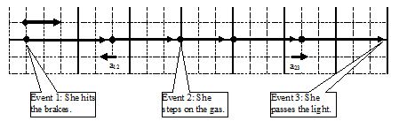
I’ve noted on the motion diagram the important events that take place during the motion. Notice that between the instant she hits the brakes and the instant she steps on the gas the acceleration is negative, while between the instant she steps on the gas and the instant she passes the light the acceleration is positive. Thus, in tabulating the motion information and applying the kinematic relations we will have to be careful not to confuse kinematic variables between these two intervals. Below is a tabulation of motion information using the coordinate system established in the motion diagram.
| Event 1: She hits the brakes. t1 = 0 s r1 = 0 m v1 = +15 m/s a12 = | Event 2: She steps on the gas. t2 = r2 = +20 m v2 = +8.0 m/s a23 = | Event 3: She passes the light t3 = r3 = +30 m v3 = +15 m/s |
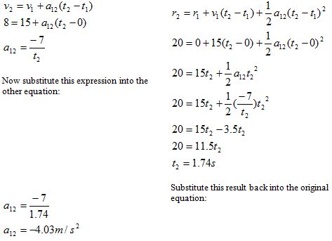
First, notice that during the time interval between “hitting the brakes” and “stepping on the gas” there are two kinematic variables that are unknown. Recall that by using your two kinematic relations, you should be able to determine these values. Second, notice that during the second time interval again two variables are unknown. Once again, the two kinematic relations will allow you to determine these values. Thus, before I actually begin to do the algebra, I know the unknown variables can be determined!
First let’s examine the motion between hitting the brakes and stepping on the gas:
Now, using these results, examine the kinematics between stepping on the gas and passing the light. Note that the initial values of the kinematic variables are denoted by ‘2’ and the final values by ‘3’, since we are examining the interval between event 2 and event 3.
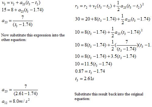
We now have a complete kinematic description of the motion.