
02. Using the Calculus


- Last updated
- Oct 1, 2024
- Save as PDF

( \newcommand{\kernel}{\mathrm{null}\,}\)
Using The Calculus
Investigate the scenario described below.
In a 100 m dash, detailed video analysis indicates that a particular sprinter’s speed can be modeled as a quadratic function of time at the beginning of the race, reaching 10.6 m/s in 2.70 s, and as a decreasing linear function of time for the remainder of the race. She finished the race in 12.6 seconds.
To analyze this situation, we should first carefully determine and define the sequence of events that take place. At each of these instants, let’s tabulate what we know about the motion.
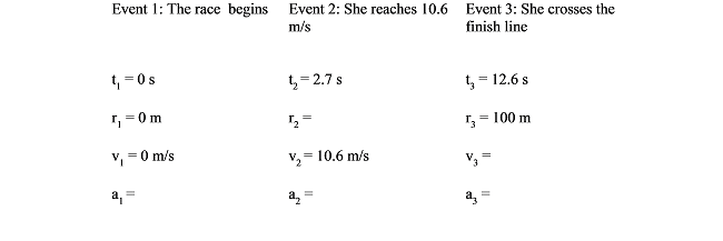
Since the acceleration is no longer necessarily constant between instants of interest, it is no longer useful to speak of a12 or a23. The acceleration, like the position and the velocity, is a function. What the table represents is the value of that function at specific instants of time.
Between event 1 and 2, the sprinter’s velocity can be modeled by a generic quadratic function of time, or

Our job is to first determine (if possible) the arbitrary constants A and B, and then use this velocity function to find the position and acceleration functions.
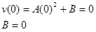
Since the sprinter starts from rest, we can evaluate the function at t = 0 s and set the result equal to 0 m/s:
Since we also know the sprinter reaches a speed of 10.6 m/s in 2.7 s, we can evaluate the function at t = 2.7 s and set the result equal to 10.6 m/s:
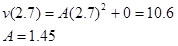
Now that we know the two constants in the velocity function, we have a complete description of the sprinter’s speed during this time interval:

Once the velocity function is determined, we differentiate to determine her acceleration function.
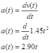
Evaluating this function at t = 0 s and t = 2.7 s yields a1 = 0 m/s2 and a2 = 7.83 m/s2.
We can also integrate to determine her position function.
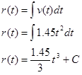
Since we know r = 0 m when t = 0 s, we can determine the integration constant:
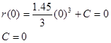
Therefore, the position of the sprinter is given by the function:

Evaluating this function at t = 0 s and t = 2.7 s yields r1 = 0 m and r2 = 9.51 m.
During the second portion of the race when her speed is decreasing linearly, her acceleration is constant. Therefore, we can use the kinematic relations developed for constant acceleration, and her acceleration is simply a constant value, denoted a23.
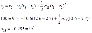

She crosses the finish line running at 7.68 m/s.