
06. The Kinematics of Circular Motion


- Last updated
- Oct 1, 2024
- Save as PDF

( \newcommand{\kernel}{\mathrm{null}\,}\)
The Kinematics of Circular Motion
Let's try out our new tools by examining the following scenario.
An automobile enters a U-turn of constant radius of curvature 95 m. The car enters the U-turn traveling at 33 m/s north and exits at 22 m/s south. Assume the speed of the car can be modeled as a quadratic function of time.
To analyze this situation, we should first carefully determine and define the sequence of events that take place. At each of these events we will tabulate the position, velocity and acceleration in polar coordinates as well as the angular position, angular velocity, and angular acceleration.
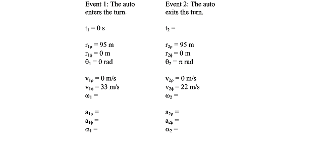
Notice that the position of the car is strictly in the radial direction and the velocity of the car is strictly in the tangential direction. It is impossible, for an object moving along a circular path, to have a non-zero tangential position or radial velocity.
Also notice that since the car completely reverses its direction of travel, it must have traveled halfway around a circular path. Thus, q2= p rad.
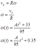
We can quickly determine the angular velocity of the car at the two events by using the relationship:

With R = 95 m, the angular velocity of the car as it enters the turn is 0.35 rad/s, and as it exits the turn, 0.23 rad/s.
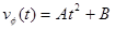
Between event 1 and 2, the car's speed can be modeled by a generic quadratic function of time, or
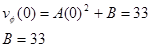
Since the car enters the turn at 33 m/s, we can evaluate the function at t = 0 s and set the result equal to 33 m/s:
The car exits the turn at 22 m/s, but since we don't know the value of t2 we can't determine A. We do know, however, that:
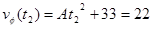
If we can determine another equation involving A and t2 we can solve these two equations simultaneously.
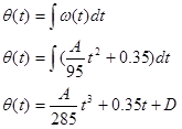
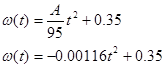
The only other important piece of information regarding the motion is that q2 = p. To make use of that information, we must "convert" our velocity equation into an angular velocity (w) equation and then integrate the resulting equation into an equation for q. To determine the angular velocity function,
The angular position (q) is the integral of the angular velocity,
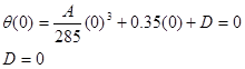
Since we know q = 0 when t = 0 s, we can determine the integration constant:
We also know that q = p at t2, so:
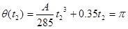
These two equations,
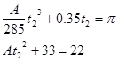
can be solved by substitution (or by using a solver). Solve the second equation for A, and substitute this expression into the first equation. You can solve the resulting equation for t2. The solution is t2 = 10.0 s, the time for the car to complete the turn. Plugging this value back into the original equation allows you to determine A = -0.11.
Once you know A, you can complete the rest of the motion table. For example, since
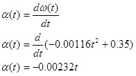
We can now determine angular acceleration,
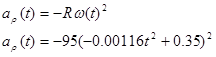
radial acceleration,
and tangential acceleration.
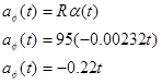
Each of these functions could be evaluted at t1 = 0 s and t2 = 10.0 s to complete the table.