
Monte Carlo Simulation
- Page ID
- 5363

\( \newcommand{\vecs}[1]{\overset { \scriptstyle \rightharpoonup} {\mathbf{#1}} } \)
\( \newcommand{\vecd}[1]{\overset{-\!-\!\rightharpoonup}{\vphantom{a}\smash {#1}}} \)
\( \newcommand{\dsum}{\displaystyle\sum\limits} \)
\( \newcommand{\dint}{\displaystyle\int\limits} \)
\( \newcommand{\dlim}{\displaystyle\lim\limits} \)
\( \newcommand{\id}{\mathrm{id}}\) \( \newcommand{\Span}{\mathrm{span}}\)
( \newcommand{\kernel}{\mathrm{null}\,}\) \( \newcommand{\range}{\mathrm{range}\,}\)
\( \newcommand{\RealPart}{\mathrm{Re}}\) \( \newcommand{\ImaginaryPart}{\mathrm{Im}}\)
\( \newcommand{\Argument}{\mathrm{Arg}}\) \( \newcommand{\norm}[1]{\| #1 \|}\)
\( \newcommand{\inner}[2]{\langle #1, #2 \rangle}\)
\( \newcommand{\Span}{\mathrm{span}}\)
\( \newcommand{\id}{\mathrm{id}}\)
\( \newcommand{\Span}{\mathrm{span}}\)
\( \newcommand{\kernel}{\mathrm{null}\,}\)
\( \newcommand{\range}{\mathrm{range}\,}\)
\( \newcommand{\RealPart}{\mathrm{Re}}\)
\( \newcommand{\ImaginaryPart}{\mathrm{Im}}\)
\( \newcommand{\Argument}{\mathrm{Arg}}\)
\( \newcommand{\norm}[1]{\| #1 \|}\)
\( \newcommand{\inner}[2]{\langle #1, #2 \rangle}\)
\( \newcommand{\Span}{\mathrm{span}}\) \( \newcommand{\AA}{\unicode[.8,0]{x212B}}\)
\( \newcommand{\vectorA}[1]{\vec{#1}} % arrow\)
\( \newcommand{\vectorAt}[1]{\vec{\text{#1}}} % arrow\)
\( \newcommand{\vectorB}[1]{\overset { \scriptstyle \rightharpoonup} {\mathbf{#1}} } \)
\( \newcommand{\vectorC}[1]{\textbf{#1}} \)
\( \newcommand{\vectorD}[1]{\overrightarrow{#1}} \)
\( \newcommand{\vectorDt}[1]{\overrightarrow{\text{#1}}} \)
\( \newcommand{\vectE}[1]{\overset{-\!-\!\rightharpoonup}{\vphantom{a}\smash{\mathbf {#1}}}} \)
\( \newcommand{\vecs}[1]{\overset { \scriptstyle \rightharpoonup} {\mathbf{#1}} } \)
\(\newcommand{\longvect}{\overrightarrow}\)
\( \newcommand{\vecd}[1]{\overset{-\!-\!\rightharpoonup}{\vphantom{a}\smash {#1}}} \)
\(\newcommand{\avec}{\mathbf a}\) \(\newcommand{\bvec}{\mathbf b}\) \(\newcommand{\cvec}{\mathbf c}\) \(\newcommand{\dvec}{\mathbf d}\) \(\newcommand{\dtil}{\widetilde{\mathbf d}}\) \(\newcommand{\evec}{\mathbf e}\) \(\newcommand{\fvec}{\mathbf f}\) \(\newcommand{\nvec}{\mathbf n}\) \(\newcommand{\pvec}{\mathbf p}\) \(\newcommand{\qvec}{\mathbf q}\) \(\newcommand{\svec}{\mathbf s}\) \(\newcommand{\tvec}{\mathbf t}\) \(\newcommand{\uvec}{\mathbf u}\) \(\newcommand{\vvec}{\mathbf v}\) \(\newcommand{\wvec}{\mathbf w}\) \(\newcommand{\xvec}{\mathbf x}\) \(\newcommand{\yvec}{\mathbf y}\) \(\newcommand{\zvec}{\mathbf z}\) \(\newcommand{\rvec}{\mathbf r}\) \(\newcommand{\mvec}{\mathbf m}\) \(\newcommand{\zerovec}{\mathbf 0}\) \(\newcommand{\onevec}{\mathbf 1}\) \(\newcommand{\real}{\mathbb R}\) \(\newcommand{\twovec}[2]{\left[\begin{array}{r}#1 \\ #2 \end{array}\right]}\) \(\newcommand{\ctwovec}[2]{\left[\begin{array}{c}#1 \\ #2 \end{array}\right]}\) \(\newcommand{\threevec}[3]{\left[\begin{array}{r}#1 \\ #2 \\ #3 \end{array}\right]}\) \(\newcommand{\cthreevec}[3]{\left[\begin{array}{c}#1 \\ #2 \\ #3 \end{array}\right]}\) \(\newcommand{\fourvec}[4]{\left[\begin{array}{r}#1 \\ #2 \\ #3 \\ #4 \end{array}\right]}\) \(\newcommand{\cfourvec}[4]{\left[\begin{array}{c}#1 \\ #2 \\ #3 \\ #4 \end{array}\right]}\) \(\newcommand{\fivevec}[5]{\left[\begin{array}{r}#1 \\ #2 \\ #3 \\ #4 \\ #5 \\ \end{array}\right]}\) \(\newcommand{\cfivevec}[5]{\left[\begin{array}{c}#1 \\ #2 \\ #3 \\ #4 \\ #5 \\ \end{array}\right]}\) \(\newcommand{\mattwo}[4]{\left[\begin{array}{rr}#1 \amp #2 \\ #3 \amp #4 \\ \end{array}\right]}\) \(\newcommand{\laspan}[1]{\text{Span}\{#1\}}\) \(\newcommand{\bcal}{\cal B}\) \(\newcommand{\ccal}{\cal C}\) \(\newcommand{\scal}{\cal S}\) \(\newcommand{\wcal}{\cal W}\) \(\newcommand{\ecal}{\cal E}\) \(\newcommand{\coords}[2]{\left\{#1\right\}_{#2}}\) \(\newcommand{\gray}[1]{\color{gray}{#1}}\) \(\newcommand{\lgray}[1]{\color{lightgray}{#1}}\) \(\newcommand{\rank}{\operatorname{rank}}\) \(\newcommand{\row}{\text{Row}}\) \(\newcommand{\col}{\text{Col}}\) \(\renewcommand{\row}{\text{Row}}\) \(\newcommand{\nul}{\text{Nul}}\) \(\newcommand{\var}{\text{Var}}\) \(\newcommand{\corr}{\text{corr}}\) \(\newcommand{\len}[1]{\left|#1\right|}\) \(\newcommand{\bbar}{\overline{\bvec}}\) \(\newcommand{\bhat}{\widehat{\bvec}}\) \(\newcommand{\bperp}{\bvec^\perp}\) \(\newcommand{\xhat}{\widehat{\xvec}}\) \(\newcommand{\vhat}{\widehat{\vvec}}\) \(\newcommand{\uhat}{\widehat{\uvec}}\) \(\newcommand{\what}{\widehat{\wvec}}\) \(\newcommand{\Sighat}{\widehat{\Sigma}}\) \(\newcommand{\lt}{<}\) \(\newcommand{\gt}{>}\) \(\newcommand{\amp}{&}\) \(\definecolor{fillinmathshade}{gray}{0.9}\)INTRODUCTION
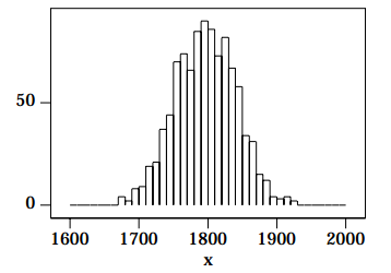
You will note that although the above shape is Gaussian, it is not perfect. Random variations occur, as they should for all Monte Carlo simulations; these random variations also occur in real data from nuclear decays.
III.B Pseudo-Random Number Generators
Consider flipping an honest coin. We say that it is random whether we get a heads or a tails, but it isn’t: in principle if we knew the initial conditions, speed and rotation of the coin, and the density and viscosity of the air and the various 2. You may wish to know that there are 1000 events, with x 0 = 1800 and σ = 44. moduli and coefficients of friction of the coin and the surface on which it lands etc. etc. we can calculate whether it will come up heads or tails. We shall call such an event pseudo-random.
Consider a single radioactive atom. The moment when it decays is usually considered to be a truly random event.3
Computers are, of course, totally deterministic (unless they are broken). This section investigates techniques to generate pseudo-random numbers using a computer. This is a huge and subtle topic, and we will only scratch the surface.
One early suggestion is due to von Neumann, one of the early giants of computer theory. In 1946 he proposed that we start with, say, a four digit number which we will call a seed.
In[1]:=
seed = 5772;
Square the number and take the middle four digits: this should be a pseudo-random number:
In[2]:= seed * seed
Out[2]= 33315984
So the pseudo-random number is 3159. Square this and take the middle four digits to generate the next pseudo-random number:
In[3]:= 3159ˆ2
Out[3]= 9979281
So the next pseudo-random number is 9792. The following code duplicates the above calculations in a more elegant fashion:
In[4]:=ran = 5772;
3. Most conventional interpretations of quantum mechanics say it is random, that "God plays dice with the universe." Recently Bohm and his school developed an interpretation of quantum mechanics which says that radioactive decay is pseudo-random.
In[5]:= ran = N[Mod[Floor[ranˆ2/10ˆ2],10ˆ4], 4]
Out[5]= 3159.
In[6]:= ran = N[Mod[Floor[ranˆ2/10ˆ2],10ˆ4], 4]
Out[6]= 9792.
Floor[] rounds its argument down to an integer; Mod[] divides its first argument by the second and returns the remainder.
Next we start with a seed of 4938 and generate 20 numbers:
In[7]:= ran = 4938;
In[8]:= Table[ ran = N[Mod[Floor[ranˆ2/10ˆ2],10ˆ4], 4], {20}]
Out[8]= {3838., 7302., 3192., 1888., 5645., 8660., 9956., 1219., 4859., 6098., 1856., 4447., 7758., 1865., 4782., 8675., 2556., 5331., 4195., 5980.}
Repeat starting with a different seed:
In[9]:= ran = 9792;
In[10]:= Table[ ran = N[Mod[Floor[ranˆ2/10ˆ2],10ˆ4], 4], {20}]
Out[10]= {8832., 42., 17., 2., 0, 0, 0, 0, 0, 0, 0, 0, 0, 0, 0, 0, 0, 0, 0, 0}
This doesn’t look too promising. Try another seed:
In[11]:= ran = 6372;
In[12]:= Table[ ran = N[Mod[Floor[ranˆ2/10ˆ2],10ˆ4], 4], {20}]
Out[12]= {6023., 2765., 6452., 6283., 4760., 6576., 2437., 9389., 1533., 3500., 2500., 2500., 2500., 2500., 2500., 2500., 2500., 2500., 2500., 2500.}
We conclude that von Neumann’s idea is poor. Mathematica’s random number generator, Random[], by default generates pseudo-random numbers between zero and one. This is a common convention. Many pseudo-random number generators, including Mathematica’s, by default choose a seed based on the time of day. One may start with a specific seed with:
SeedRandom[ seed ]
and Random[] will then generate identical sequences of numbers:
In[13]:= SeedRandom[1234];
In[14]:= Table[Random[], {10}]
Out[14]= {0.681162, 0.854217, 0.432088, 0.897439, 0.890045, 0.48555, 0.555124, 0.0837, 0.0108901, 0.309357}
In[15]:= Table[Random[], {10}]
Out[15]= {0.626772, 0.230746, 0.430667, 0.764379, 0.809171, 0.476566, 0.643232, 0.542694, 0.565734, 0.208041}
In[16]:= SeedRandom[1234];
In[17]:= Table[Random[], {10}]
Out[17]= {0.681162, 0.854217, 0.432088, 0.897439, 0.890045, 0.48555, 0.555124, 0.0837, 0.0108901, 0.309357}
In[18]:= Table[Random[], {10}]
Out[18]= {0.626772, 0.230746, 0.430667, 0.764379, 0.809171, 0.476566, 0.643232, 0.542694, 0.565734, 0.208041}
All pseudo-random number generators have a non-infinite period: sooner or later the numbers in the sequences will repeat. A good generator will have a period that is sufficiently long that for practical purposes the numbers will never repeat. Most generators today are variations on a linear congruential algorithm. Calling the seed X0, the algorithm is:
\[X_{n +1} = Mod[aX_n + c, m] \]
where:
m > 0
0 ≤ a < m
0 ≤ c < m
The choices for m, a and c is subtle. For example, if m = 10 and X0 = a = c = 7, the generator has a period of only four numbers:
7, 6, 9, 0, 7, 6, 9, 0, ...
The UNIX random number generator rand() has a period of 232.
In addition to the rather arcane theory of random number generation, people have devised a variety of methods to test the generators. Knuth4 lists 11 empirical tests. In the experiment you will use only one of them: the equidistribution test. In this test you check that the random numbers are in fact uniformly distributed between the minimum and maximum values.
IV. REFERENCES
• D.E. Knuth The Art of Computer Programming, 2nd ed. (Addison-Wesley, 1973), Vol 2, Chapter 3. This is a classic seven volume work. The cited chapter deals with computer generated random numbers.
• William H. Press, Brian P. Flannery, Saul A. Teukolsky, and William T. Vetterling, Numerical Recipes: The Art of Scientific Computing or Numerical Recipes in C: The Art of Scientific Computing (Cambridge Univ. Press), §14.5 (Confidence Limits) and Chapt. 7 (Random Numbers. A thorough discussion of confidence limits and Monte Carlo techniques.
• E.F. Taylor and J.A. Wheeler Spacetime Physics (W.H. Freeman, 1963). My personal favorite book on relativity.