11.1: The Driven Harmonic Oscillator

As an introduction to the Green’s function technique, we will study the driven harmonic oscillator, which is a damped harmonic oscillator subjected to an arbitrary driving force. The equation of motion is \[\left[\frac{d^2}{dt^2} + 2 \gamma \frac{d}{dt} + \omega_0^2\right] x(t) = \frac{f(t)}{m}.\] Here, \(m\) is the mass of the particle, \(\gamma\) is the damping coefficient, and \(\omega_0\) is the natural frequency of the oscillator. The left side of the equation is the same as in the damped harmonic oscillator equation (see Chapter 5). On the right side, we introduce a time-dependent driving force \(f(t)\), which acts alongside the pre-existing spring and damping forces. Given an arbitrarily complicated \(f(t)\), our goal is to determine \(x(t)\).

Green’s function for the driven harmonic oscillator

Prior to solving the driven harmonic oscillator problem for a general driving force \(f(t)\), let us first consider the following equation: \[\left[\frac{\partial^2}{\partial t^2} + 2 \gamma \frac{\partial}{\partial t} + \omega_0^2\right] G(t, t') = \delta(t-t'). \label{greenfuneq}\] The function \(G(t,t')\), which depends on the two variables \(t\) and \(t'\), is called the Green’s function. Note that the differential operator on the left side involves only derivatives in \(t\).

The Green’s function describes the motion of a damped harmonic oscillator subjected to a particular driving force that is a delta function, describing an infinitesimally sharp pulse centered at \(t = t'\): \[\frac{f(t)}{m} = \delta(t-t').\] Here’s the neat thing about \(G(t,t')\): once we know it, we can find a specific solution to the driven harmonic oscillator equation for any \(f(t)\). The solution has the form \[x(t) = \int^\infty_{-\infty} dt' \; G(t,t') \; \frac{f(t')}{m}.\] To show that this is indeed a solution, plug it into the equation of motion: \[\begin{align} \left[\frac{d^2}{dt^2} + 2 \gamma \frac{d}{dt} + \omega_0^2\right]\, x(t) &= \int^\infty_{-\infty} dt' \; \left[\frac{\partial^2}{\partial t^2} + 2 \gamma \frac{\partial}{\partial t} + \omega_0^2\right] G(t,t') \frac{f(t')}{m} \\ &= \int^\infty_{-\infty} dt' \; \delta(t-t')\, \frac{f(t')}{m} \\ &= \frac{f(t)}{m}.\end{align}\] Note that we can move the differential operator inside the integral because \(t\) and \(t'\) are independent variables.

The Green’s function concept is based on the principle of superposition. The motion of the oscillator is induced by the driving force, but the value of \(x(t)\) at time \(t\) does not depend only on the instantaneous value of \(f(t)\) at time \(t\); instead, it depends on the values of \(f(t')\) over all past times \(t' < t\). We can thus decompose \(f\) into a superposition of pulses described by delta functions at different times. Then \(x(t)\) is a superposition of the oscillations produced by the individual pulses.

Finding the Green’s function

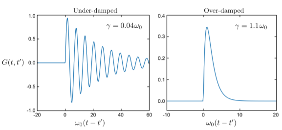
To find the Green’s function, we can use the Fourier transform. Let us assume that the Fourier transform of \(G(t,t')\) with respect to \(t\) is convergent, and that the oscillator is not critically damped (i.e., \(\omega_0 \ne \gamma\); see Section 5.3). The Fourier transformation of the Green’s function (also called the frequency-domain Green’s function) is \[G(\omega, t') = \int_{-\infty}^\infty dt \; e^{i\omega t}\, G(t,t').\] Here, we have used the sign convention for time-domain Fourier transforms (see Section 10.3). Applying the Fourier transform to both sides of the Green’s function equation, and making use of how derivatives behave under Fourier transformation (see Section 10.4), gives \[\left[- \omega^2 - 2i \gamma\omega + \omega_0^2\right] G(\omega,t') = \int_{-\infty}^\infty dt \; e^{i\omega t}\, \delta(t-t') = e^{i\omega t'}. \label{green-omega}\] The differential equation for \(G(t,t')\) has thus been converted into an algebraic equation for \(G(\omega,t')\), whose solution is \[G(\omega, t') = - \frac{e^{i\omega t'}}{\omega^2 + 2i\gamma\omega - \omega_0^2}.\] Finally, we retrieve the time-domain solution by using the inverse Fourier transform: \[\begin{align} G(t,t') &= \int_{-\infty}^\infty \frac{d\omega}{2\pi} \, e^{-i\omega t} G(\omega, t') \\ &= - \int_{-\infty}^\infty \frac{d\omega}{2\pi} \, \frac{e^{-i\omega (t-t')}}{\omega^2 + 2i\gamma\omega - \omega_0^2}.\end{align}\] The denominator of the integral is a quadratic expression, so this can be re-written as: \[G(t,t') = - \int_{-\infty}^\infty \frac{d\omega}{2\pi} \, \frac{e^{-i\omega (t-t')}}{(\omega - \omega_+)(\omega - \omega_-)} \quad\mathrm{where}\;\; \omega_{\pm} = -i\gamma \pm \sqrt{\omega_0^2-\gamma^2}.\] This can be evaluated by contour integration. The integrand has two poles, which are precisely the complex frequencies of the damped harmonic oscillator; both lie in the negative complex plane. For \(t < t'\), Jordan’s lemma requires us to close the contour in the upper half-plane, enclosing neither pole, so the integral is zero. For \(t > t'\), we must close the contour in the lower half-plane, enclosing both poles, so the result is \[\begin{align} G(t,t') &= i \Theta(t-t') \, \left[ \frac{e^{-i\omega_+ (t-t')}}{\omega_+ - \omega_- } + \frac{e^{-i\omega_- (t-t')}}{\omega_- - \omega_+}\right] \\ &= \Theta(t-t') \;e^{-\gamma(t-t')} \; \times \left\{\begin{array}{ll} \frac{1}{\sqrt{\omega_0^2-\gamma^2}}\, \sin\left[\sqrt{\omega_0^2-\gamma^2} (t-t')\right], & \gamma < \omega_0, \\ \frac{1}{\sqrt{\gamma^2-\omega_0^2}}\, \sinh\left[\sqrt{\gamma^2-\omega_0^2} (t-t')\right], & \gamma > \omega_0. \end{array}\right. \label{greensol}\end{align}\] Here, \(\Theta(t-t')\) refers to the step function \[\Theta(\tau) = \left\{\begin{array}{ll} 1, &\;\;\;\textrm{for} \; \tau \ge 0\\ 0,&\;\;\; \textrm{otherwise.}\end{array}\right.\] The result is plotted in the figure below for two different choices of \(\gamma\) and \(\omega_0\). The solution for the critically damped case, \(\gamma = \omega_0\), is left as an exercise.

Figure \(\PageIndex{1}\)

Features of the Green’s function

As previously noted, the time-domain Green’s function has a physical meaning: it represents the motion of the oscillator in response to a pulse of force, \(f(t) = m\, \delta(t-t')\). Let us examine the result obtained in the previous section in greater detail, to see if it matches our physical intuition.

The first thing to notice is that the Green’s function depends on \(t\) and \(t'\) only in the combination \(t-t'\). This makes sense: the response of the oscillator to the force pulse should only depend on the time elapsed since the pulse. We can take advantage of this property by re-defining the frequency-domain Green’s function as \[G(\omega) = \int_{-\infty}^\infty dt \; e^{i\omega (t-t')}\, G(t-t'),\] which then obeys \[\left[- \omega^2 - 2i \gamma\omega + \omega_0^2\right] G(\omega) = 1.\] This is nicer to work with than Eq. \(\eqref{green-omega}\) as there is no extraneous \(t'\) variable present.

Next, note how the Green’s function behaves just before and after the pulse. Its value is zero for all \(t - t' < 0\) (i.e., prior to the pulse). This feature will be discussed in greater detail in the next section. Moreover, there is no discontinuity in \(x(t)\) at \(t - t' = 0\); the force pulse does not cause the oscillator to “teleport” instantaneously to a different position. Instead, it produces a discontinuity in the oscillator’s velocity.

We can calculate the velocity discontinuity by integrating the Green’s function equation over an infinitesimal interval of time surrounding \(t'\): \[\begin{align} \lim_{\epsilon \rightarrow 0} \int_{t'-\epsilon}^{t'+\epsilon} dt \left[\frac{\partial^2}{\partial t^2} + 2\gamma\frac{\partial}{\partial t} + \omega_0^2\right] G(t,t') &= \lim_{\epsilon \rightarrow 0} \int_{t'-\epsilon}^{t'+\epsilon} dt \; \delta(t-t') \\ = \lim_{\epsilon \rightarrow 0} \left\{ \left.\frac{\partial G(t,t')}{\partial t}\right|_{t = t' +\epsilon} - \left.\frac{\partial G(t,t')}{\partial t}\right|_{t = t' - \epsilon}\right\} &= 1.\end{align}\] On the last line, the expression on the left-hand side represents the difference between the velocities just after and before the pulse. Evidently, the pulse imparts one unit of velocity at \(t=t'\). Looking at the solutions obtained in Section 11.1, we can verify that \(\partial G/\partial t = 0\) right before the pulse, and \(\partial G/\partial t = 1\) right after it.

For \(t - t' > 0\), the applied force goes back to zero, and the system behaves like the undriven harmonic oscillator. If the oscillator is under-damped (\(\gamma < \omega_0\)), it undergoes a decaying oscillation around the origin. If the oscillator is over-damped (\(\gamma > \omega_0\)), it moves ahead for a distance, then settles exponentially back to the origin.

Causality

We have seen that the motion \(x(t)\) ought to depend on the driving force \(f(t')\) at all past times \(t' < t\), but should not depend on the force at future times. Because of the relation \[x(t) = \int_{-\infty}^\infty dt'\; G(t,t')\, \frac{f(t')}{m},\] this means that the Green’s function ought to satisfy \[G(t,t') = 0 \;\; \mathrm{for}\;\; t -t' < 0.\] This condition is referred to as causality, because it is equivalent to saying that cause must precede effect. A Green’s function with this feature is called a causal Green’s function.

For the driven harmonic oscillator, the time-domain Green’s function satisfies a second-order differential equation, so its general solution must contain two free parameters. The specific solution that we derived above, Eq. \(\eqref{greensol}\), turns out to be the only causal solution. There are a couple of ways to see why.

The first way is to observe that for \(t > t'\), the Green’s function satisfies the differential equation for the undriven harmonic oscillator. But based on the discussion in Section 11.1, the causal Green’s function needs to obey two conditions at \(t = t' + 0^+\): (i) \(G = 0\), and (ii) \(\partial G / \partial t = 1\). These act as two boundary conditions for the undriven harmonic oscillator equation, giving rise to the specific solution that we found.

The other way to see that the causal Green’s function is unique is to imagine adding to our specific solution any solution \(x_1(t)\) for the undriven harmonic oscillator. It is easily verified that the resulting \(G(t,t')\) is also a solution to Eq. \(\eqref{greenfuneq}\). Since the general solution for \(x_1(t)\) contains two free parameters, we have thus found the general solution for \(G(t,t')\). But the solutions for \(x_1(t)\) are all infinite in the \(t \rightarrow -\infty\) limit, except for the trivial solution \(x_1(t) = 0\). That choice corresponds to the causal Green’s function \(\eqref{greensol}\).