
7.2: Discretizing Partial Differential Equations


- Last updated
- Apr 30, 2021
- Save as PDF

( \newcommand{\kernel}{\mathrm{null}\,}\)
With discretized derivatives, differential equations can be formulated as discrete systems of equations. We will discuss this using a specific example: the discretization of the time-independent Schrödinger wave equation in 1D.
7.2.1 Deriving a Finite-Difference Equation
The 1D time-independent Schrödinger wave equation is the second-order ordinary differential equation
−ℏ22md2ψdx2+V(x)ψ(x)=Eψ(x),
where ℏ is Planck's constant divided by 2π, m is the mass of the particle, V(x) is the potential, ψ(x) is the quantum wavefunction of an energy eigenstate of the particle, and E is the corresponding energy. The differential equation is usually treated as an eigenproblem, in the sense that we are given V(x) and seek to find the possible values of the eigenfunction ψ(x) and the energy eigenvalue E. For convenience, we will adopt units where ℏ=m=1:
−12d2ψdx2+V(x)ψ(x)=Eψ(x).
To discretize this differential equation, we simply evaluate it at x=xn:
−12ψ″(xn)+Vnψn=Eψn,
where, for conciseness, we denote
Vn≡V(xn).
We then replace the second derivative ψ″(xn) with a discrete approximation, specifically the three-point rule:
−12h2[ψn+1−2ψn+ψn−1]+Vnψn=Eψn.
This result is called a finite-difference equation, and it would be valid for all n if the number of discretization points is infinite. However, if there is a finite number of discretization points, {x0,x1,…,xN−1}, then the finite-difference formula fails at the boundary points, n=0 and n=N−1, where it involves the value of the function at the "non-existent" points x−1 and xN. We'll see how to handle this problem in the next section.
Boundaries aside, the finite-difference equation describes a matrix equation:
{−12h2[⋱⋱⋱−211−211−2⋱⋱⋱]+[⋱Vn−1VnVn+1⋱]}[⋮ψn−1ψnψn+1⋮]=E[⋮ψn−1ψnψn+1⋮].
The second-derivative operator is represented by a tridiagonal matrix with −2 in each diagonal element, and 1 in the elements directly above and below the diagonal. The potential operator is represented by a diagonal matrix, where the elements along the diagonal are the values of the potential at each discretization point. In this way, the Schrödinger wave equation is reduced to a discrete eigenvalue problem.
7.2.2 Boundary Conditions
We now have to figure out how to handle the boundaries. Let us suppose ψ(x) is defined over a finite interval, a≤x≤b. As we recall from the theory of differential equations, the solution to a differential equation is not wholly determined by the differential equation itself, but also by the boundary conditions that are imposed. Thus, we have to specify how ψ(x) behaves at the end-points of the interval. We will show how this is done for a couple of the most common boundary conditions; other choices of boundary conditions can be handled using the same kind of reasoning.
Dirichlet Boundary Conditions
Under Dirichlet boundary conditions, the wavefunction vanishes at the boundaries:
ψ(a)=ψ(b)=0.
Physically, these boundary conditions apply if we let the potential blow up in the external regions, x>b and x<a, thus forcing the wavefunction to be strictly confined to the interval a≤x≤b.
We have not yet stated how the discretization points {x0,…,xN−1} are distributed within the interval; we will make this decision in tandem with the implementation of the boundary conditions. Consider the first discretization point, x0, wherever it is. The finite-difference equation at this point is
−12h2[ψ−1−2ψ0+ψ1]+V0ψ0=Eψ0.
This involves the wavefunction at x−1, which lies just outside our set of discretization points. But if we choose the discretization points so that x−1=a, then ψ−1=0 under Dirichlet boundary conditions, so the above finite-difference formula reduces to
−12h2[−2ψ0+ψ1]+V0ψ0=Eψ0.
As for the other boundary, the finite-difference equation at xN−1 involves ψN. If we choose the discretization points so that xN=b, then the finite-difference formula becomes
−12h2[ψN−2−2ψN−1]+VN−1ψN−1=EψN−1.
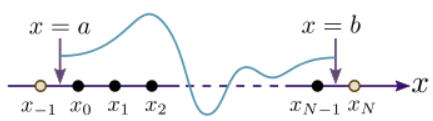
From this, we conclude that the discretization points ought to be equally spaced, with x0 at a distance h to the right of the left boundary a and xN−1 a distance h to the left of the right boundary b. This is shown in the following figure:

Since there are N discretization points, the interval should contain (N+1) multiples of h. Hence,
h=b−aN+1⇒xn=a+h(n+1)=a(N−n)+b(n+1)N+1.
Having made the above choices, the matrix equation becomes
{−12h2[−211−2⋱⋱⋱11−2]+[V0V1⋱VN−1]}[ψ0ψ1⋮ψN−1]=E[ψ0ψ1⋮ψN−1].
You can check for yourself that the first and last rows of this equation are the correct finite-difference equations at the boundary points, corresponding to Dirichlet boundary conditions.
Neuman boundary conditions
Neumann boundary conditions are another common choice of boundary conditions. They state that the first derivatives vanish at the boundaries:
ψ′(a)=ψ′(b)=0.
An example of such a boundary condition is encountered in electrostatics, where the first derivative of the electric potential goes to zero at the surface of a charged metallic surface.
We follow the same strategy as before, figuring out the discretization points in tandem with the boundary conditions. Consider again the finite-difference equation at the first discretization point:
−12h2[ψ−1−2ψ0+ψ1]+V0ψ0=Eψ0.
To implement the condition that first derivative vanishes at the boundary, we invoke the mid-point rule. Suppose the boundary point x=a falls in between the points x−1 and x0. Then, according to the mid-point rule,
ψ0−ψ−1h≈ψ′(a)=0.
With this choice, therefore, we can make the replacement ψ−1=ψ0 in the finite-difference equation, which then becomes
−12h2[−ψ0+ψ1]+V0ψ0=Eψ0.
Similarly, to apply the Neumann boundary condition at x=b, we let the boundary fall between xN−1 and xN, so that the finite-difference equation becomes
−12h2[ψN−2−ψN−1]+VN−1ψN−1=EψN−1.
The resulting distribution of discretization points is shown in the following figure:
Unlike the Dirichlet case, the interval contains N multiples of h. Hence, we get a different formula for the positions of the discretization points
h=b−aN⇒xn=a+h(n+12)=a(N−n−12)+b(n+12)N.
The matrix equation is:
{−12h2[−111−2⋱⋱⋱⋱⋱−211−1]+[V0V1⋱VN−1]}[ψ0ψ1⋮ψN−1]=E[ψ0ψ1⋮ψN−1].
Due to the Neumann boundary conditions and the mid-point rule, the tridiagonal matrix has −1 instead of −2 on its corner entries. Again, you can verify that the first and last rows of this matrix equation correspond to the correct finite-difference equations for the boundary points.