
2.5: Operators, Commutators and Uncertainty Principle
- Page ID
- 25700

Commutator
The Commutator of two operators A, B is the operator C = [A, B] such that C = AB − BA.
If the operators A and B are scalar operators (such as the position operators) then AB = BA and the commutator is always zero.
If the operators A and B are matrices, then in general \( A B \neq B A\). Consider for example:
\[A=\frac{1}{2}\left(\begin{array}{ll}
0 & 1 \\
1 & 0
\end{array}\right), \quad B=\frac{1}{2}\left(\begin{array}{cc}
1 & 0 \\
0 & -1
\end{array}\right) \nonumber\]
Then
\[A B=\frac{1}{2}\left(\begin{array}{cc}
0 & -1 \\
1 & 0
\end{array}\right), \quad B A=\frac{1}{2}\left(\begin{array}{cc}
0 & 1 \\
-1 & 0
\end{array}\right) \nonumber\]
Then [A, B] = 2AB.
A is Turn to your right. B is Take 3 steps to your left.
Question
Do these two operators commute?
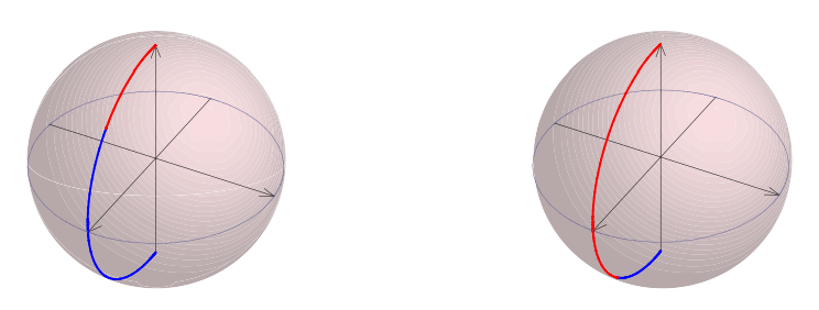
Let A and B be two rotations. First assume that A is a \(\pi\)/4 rotation around the x direction and B a 3\(\pi\)/4 rotation in the same direction. Now assume that the vector to be rotated is initially around z. Then, if we apply AB (that means, first a 3\(\pi\)/4 rotation around x and then a \(\pi\)/4 rotation), the vector ends up in the negative z direction. The same happen if we apply BA (first A and then B).
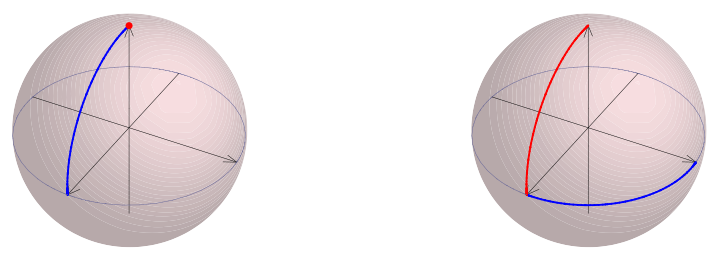
Now assume that A is a \(\pi\)/2 rotation around the x direction and B around the z direction. When we apply AB, the vector ends up (from the z direction) along the y-axis (since the first rotation does not do anything to it), if instead we apply BA the vector is aligned along the x direction. In this case the two rotations along different axes do not commute.
These examples show that commutators are not specific of quantum mechanics but can be found in everyday life. We now want an example for QM operators.
The most famous commutation relationship is between the position and momentum operators. Consider first the 1D case. We want to know what is \(\left[\hat{x}, \hat{p}_{x}\right] \) (I’ll omit the subscript on the momentum). We said this is an operator, so in order to know what it is, we apply it to a function (a wavefunction). Let’s call this operator \(C_{x p}, C_{x p}=\left[\hat{x}, \hat{p}_{x}\right]\).
\[[\hat{x}, \hat{p}] \psi(x)=C_{x p}[\psi(x)]=\hat{x}[\hat{p}[\psi(x)]]-\hat{p}[\hat{x}[\psi(x)]]=-i \hbar\left(x \frac{d}{d x}-\frac{d}{d x} x\right) \psi(x) \nonumber\]
\[-i \hbar\left(x \frac{d \psi(x)}{d x}-\frac{d}{d x}(x \psi(x))\right)=-i \hbar\left(x \frac{d \psi(x)}{d x}-\psi(x)-x \frac{d \psi(x)}{d x}\right)=i \hbar \psi(x) \nonumber\]
From \([\hat{x}, \hat{p}] \psi(x)=i \hbar \psi(x) \) which is valid for all \( \psi(x)\) we can write
\[\boxed{[\hat{x}, \hat{p}]=i \hbar }\nonumber\]
Considering now the 3D case, we write the position components as \(\left\{r_{x}, r_{y} r_{z}\right\} \). Then we have the commutator relationships:
\[\boxed{\left[\hat{r}_{a}, \hat{p}_{b}\right]=i \hbar \delta_{a, b} }\nonumber\]
that is, vector components in different directions commute (the commutator is zero).
Properties of commutators
- Any operator commutes with scalars \([A, a]=0\)
- [A, BC] = [A, B]C + B[A, C] and [AB, C] = A[B, C] + [A, C]B
- Any operator commutes with itself [A, A] = 0, with any power of itself [A, An] = 0 and with any function of itself \([A, f(A)]=0\) (from previous property and with power expansion of any function).
From these properties, we have that the Hamiltonian of the free particle commutes with the momentum: \([p, \mathcal{H}]=0 \) since for the free particle \( \mathcal{H}=p^{2} / 2 m\). Also, \(\left[x, p^{2}\right]=[x, p] p+p[x, p]=2 i \hbar p \).
We now prove an important theorem that will have consequences on how we can describe states of a systems, by measuring different observables, as well as how much information we can extract about the expectation values of different observables.
If A and B commute, then they have a set of non-trivial common eigenfunctions.
- Proof
-
Let \(\varphi_{a}\) be an eigenfunction of A with eigenvalue a:
\[A \varphi_{a}=a \varphi_{a} \nonumber\]
Then
\[B A \varphi_{a}=a B \varphi_{a} \nonumber\]
But since [A, B] = 0 we have BA = AB. Let’s substitute in the LHS:
\[A\left(B \varphi_{a}\right)=a\left(B \varphi_{a}\right) \nonumber\]
This means that (\( B \varphi_{a}\)) is also an eigenfunction of A with the same eigenvalue a. If \(\varphi_{a}\) is the only linearly independent eigenfunction of A for the eigenvalue a, then \( B \varphi_{a}\) is equal to \( \varphi_{a}\) at most up to a multiplicative constant: \( B \varphi_{a} \propto \varphi_{a}\).
That is, we can write
\[B \varphi_{a}=b_{a} \varphi_{a} \nonumber\]
But this equation is nothing else than an eigenvalue equation for B. Then \( \varphi_{a}\) is also an eigenfunction of B with eigenvalue \( b_{a}\). We thus proved that \( \varphi_{a}\) is a common eigenfunction for the two operators A and B. ☐
We have just seen that the momentum operator commutes with the Hamiltonian of a free particle. Then the two operators should share common eigenfunctions.
This is indeed the case, as we can verify. Consider the eigenfunctions for the momentum operator:
\[\hat{p}\left[\psi_{k}\right]=\hbar k \psi_{k} \quad \rightarrow \quad-i \hbar \frac{d \psi_{k}}{d x}=\hbar k \psi_{k} \quad \rightarrow \quad \psi_{k}=A e^{-i k x} \nonumber\]
What is the Hamiltonian applied to \( \psi_{k}\)?
\[\mathcal{H}\left[\psi_{k}\right]=-\frac{\hbar^{2}}{2 m} \frac{d^{2}\left(A e^{-i k x}\right)}{d x^{2}}=\frac{\hbar^{2} k^{2}}{2 m} A e^{-i k x}=E_{k} \psi_{k} \nonumber\]
thus we found that \(\psi_{k} \) is also a solution of the eigenvalue equation for the Hamiltonian, which is to say that it is also an eigenfunction for the Hamiltonian.
Commuting observables
Degeneracy
In the proof of the theorem about commuting observables and common eigenfunctions we took a special case, in which we assume that the eigenvalue \(a\) was non-degenerate. That is, we stated that \(\varphi_{a}\) was the only linearly independent eigenfunction of A for the eigenvalue \(a\) (functions such as \(4 \varphi_{a}, \alpha \varphi_{a} \) don’t count, since they are not linearly independent from \(\varphi_{a} \)).
In general, an eigenvalue is degenerate if there is more than one eigenfunction that has the same eigenvalue. The degeneracy of an eigenvalue is the number of eigenfunctions that share that eigenvalue.
For example \(a\) is \(n\)-degenerate if there are \(n\) eigenfunction \( \left\{\varphi_{j}^{a}\right\}, j=1,2, \ldots, n\), such that \( A \varphi_{j}^{a}=a \varphi_{j}^{a}\).
What happens if we relax the assumption that the eigenvalue \(a\) is not degenerate in the theorem above? Consider for example that there are two eigenfunctions associated with the same eigenvalue:
\[A \varphi_{1}^{a}=a \varphi_{1}^{a} \quad \text { and } \quad A \varphi_{2}^{a}=a \varphi_{2}^{a} \nonumber\]
then any linear combination \(\varphi^{a}=c_{1} \varphi_{1}^{a}+c_{2} \varphi_{2}^{a} \) is also an eigenfunction with the same eigenvalue (there’s an infinity of such eigenfunctions). From the equality \(A\left(B \varphi^{a}\right)=a\left(B \varphi^{a}\right)\) we can still state that (\( B \varphi^{a}\)) is an eigenfunction of A but we don’t know which one. Most generally, there exist \(\tilde{c}_{1}\) and \(\tilde{c}_{2}\) such that
\[B \varphi_{1}^{a}=\tilde{c}_{1} \varphi_{1}^{a}+\tilde{c}_{2} \varphi_{2}^{a} \nonumber\]
but in general \( B \varphi_{1}^{a} \not \alpha \varphi_{1}^{a}\), or \(\varphi_{1}^{a} \) is not an eigenfunction of B too.
Consider again the energy eigenfunctions of the free particle. To each energy \(E=\frac{\hbar^{2} k^{2}}{2 m} \) are associated two linearly-independent eigenfunctions (the eigenvalue is doubly degenerate). We can choose for example \( \varphi_{E}=e^{i k x}\) and \(\varphi_{E}=e^{-i k x} \). Notice that these are also eigenfunctions of the momentum operator (with eigenvalues ±k). If we had chosen instead as the eigenfunctions cos(kx) and sin(kx) these are not eigenfunctions of \(\hat{p}\).
In general, it is always possible to choose a set of (linearly independent) eigenfunctions of A for the eigenvalue \(a\) such that they are also eigenfunctions of B.
For the momentum/Hamiltonian for example we have to choose the exponential functions instead of the trigonometric functions. Also, if the eigenvalue of A is degenerate, it is possible to label its corresponding eigenfunctions by the eigenvalue of B, thus lifting the degeneracy. For example, there are two eigenfunctions associated with the energy E: \(\varphi_{E}=e^{\pm i k x} \). We can distinguish between them by labeling them with their momentum eigenvalue \(\pm k\): \( \varphi_{E,+k}=e^{i k x}\) and \(\varphi_{E,-k}=e^{-i k x} \).
- Proof
-
Assume now we have an eigenvalue \(a\) with an \(n\)-fold degeneracy such that there exists \(n\) independent eigenfunctions \(\varphi_{k}^{a}\), k = 1, . . . , n. Any linear combination of these functions is also an eigenfunction \(\tilde{\varphi}^{a}=\sum_{k=1}^{n} \tilde{c}_{k} \varphi_{k}^{a}\). For any of these eigenfunctions (let’s take the \( h^{t h}\) one) we can write:
\[B\left[A\left[\varphi_{h}^{a}\right]\right]=A\left[B\left[\varphi_{h}^{a}\right]\right]=a B\left[\varphi_{h}^{a}\right] \nonumber\]
so that \( \bar{\varphi}_{h}^{a}=B\left[\varphi_{h}^{a}\right]\) is an eigenfunction of A with eigenvalue a. Then this function can be written in terms of the \( \left\{\varphi_{k}^{a}\right\}\):
\[B\left[\varphi_{h}^{a}\right]=\bar{\varphi}_{h}^{a}=\sum_{k} \bar{c}_{h, k} \varphi_{k}^{a} \nonumber\]
This notation makes it clear that \( \bar{c}_{h, k}\) is a tensor (an n × n matrix) operating a transformation from a set of eigenfunctions of A (chosen arbitrarily) to another set of eigenfunctions. We can write an eigenvalue equation also for this tensor,
\[\bar{c} v^{j}=b^{j} v^{j} \quad \rightarrow \quad \sum_{h} \bar{c}_{h, k} v_{h}^{j}=b^{j} v^{j} \nonumber\]
where the eigenvectors \(v^{j} \) are vectors of length \( n\).
If we now define the functions \( \psi_{j}^{a}=\sum_{h} v_{h}^{j} \varphi_{h}^{a}\), we have that \( \psi_{j}^{a}\) are of course eigenfunctions of A with eigenvalue a. Also
\[B\left[\psi_{j}^{a}\right]=\sum_{h} v_{h}^{j} B\left[\varphi_{h}^{a}\right]=\sum_{h} v_{h}^{j} \sum_{k=1}^{n} \bar{c}_{h, k} \varphi_{k}^{a} \nonumber\]
\[=\sum_{k} \varphi_{k}^{a} \sum_{h} \bar{c}_{h, k} v_{h}^{j}=\sum_{k} \varphi_{k}^{a} b^{j} v_{k}^{j}=b^{j} \sum_{k} v_{k}^{j} \varphi_{k}^{a}=b^{j} \psi_{j}^{a} \nonumber\]
We have thus proved that \( \psi_{j}^{a}\) are eigenfunctions of B with eigenvalues \(b^{j} \). The \( \psi_{j}^{a}\) are simultaneous eigenfunctions of both A and B.
Consider the set of functions \( \left\{\psi_{j}^{a}\right\}\). From the point of view of A they are not distinguishable, they all have the same eigenvalue so they are degenerate. Taking into account a second operator B, we can lift their degeneracy by labeling them with the index j corresponding to the eigenvalue of B (\(b^{j}\)).
Assume that we choose \( \varphi_{1}=\sin (k x)\) and \( \varphi_{2}=\cos (k x)\) as the degenerate eigenfunctions of \( \mathcal{H}\) with the same eigenvalue \( E_{k}=\frac{\hbar^{2} k^{2}}{2 m}\). We now want to find with this method the common eigenfunctions of \(\hat{p} \). We first need to find the matrix \( \bar{c}\) (here a 2×2 matrix), by applying \( \hat{p}\) to the eigenfunctions.
\[ \hat{p} \varphi_{1}=-i \hbar \frac{d \varphi_{1}}{d x}=i \hbar k \cos (k x)=-i \hbar k \varphi_{2} \nonumber\]
and \( \hat{p} \varphi_{2}=i \hbar k \varphi_{1}\). Then the matrix \( \bar{c}\) is:
\[\bar{c}=\left(\begin{array}{cc}
0 & i \hbar k \\
-i \hbar k & 0
\end{array}\right) \nonumber\]
with eigenvalues \( \), and eigenvectors (not normalized)
\[v^{1}=\left[\begin{array}{l}
-i \\
1
\end{array}\right], \quad v^{2}=\left[\begin{array}{l}
i \\
1
\end{array}\right] \nonumber\]
We then write the \(\psi\) eigenfunctions:
\[\psi^{1}=v_{1}^{1} \varphi_{1}+v_{2}^{1} \varphi_{2}=-i \sin (k x)+\cos (k x) \propto e^{-i k x}, \quad \psi^{2}=v_{1}^{2} \varphi_{1}+v_{2}^{2} \varphi_{2}=i \sin (k x)+\cos (k x) \propto e^{i k x} \nonumber\]
Complete set of commuting observables
We have seen that if an eigenvalue is degenerate, more than one eigenfunction is associated with it. Then, if we measure the observable A obtaining \(a\) we still do not know what the state of the system after the measurement is. If we take another observable B that commutes with A we can measure it and obtain \(b\). We have thus acquired some extra information about the state, since we know that it is now in a common eigenstate of both A and B with the eigenvalues \(a\) and \(b\). Still, this could be not enough to fully define the state, if there is more than one state \( \varphi_{a b} \). We can then look for another observable C, that commutes with both A and B and so on, until we find a set of observables such that upon measuring them and obtaining the eigenvalues a, b, c, d, . . . the function \(\varphi_{a b c d \ldots} \) is uniquely defined. Then the set of operators {A, B, C, D, . . . } is called a complete set of commuting observables. The eigenvalues a, b, c, d, . . . that specify the state are called good quantum numbers and the state is written in Dirac notation as \(|a b c d \ldots\rangle \).
Obs. The set of commuting observable is not unique.
Uncertainty principle
Uncertainty for waves
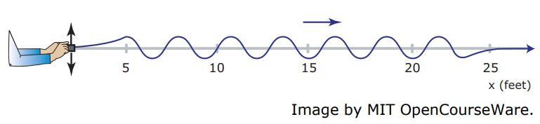
The uncertainty principle, which you probably already heard of, is not found just in QM. Consider for example the propagation of a wave. If you shake a rope rhythmically, you generate a stationary wave, which is not localized (where is the wave??) but it has a well defined wavelength (and thus a momentum).
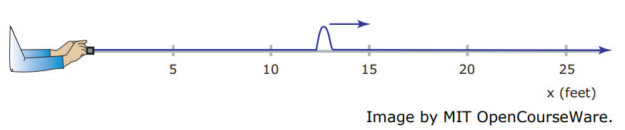
If instead you give a sudden jerk, you create a well localized wavepacket. Now however the wavelength is not well defined (since we have a superposition of waves with many wavelengths). The position and wavelength cannot thus be well defined at the same time. In QM we express this fact with an inequality involving position and momentum \( p=\frac{2 \pi \hbar}{\lambda}\). Then we have \( \sigma_{x} \sigma_{p} \geq \frac{\hbar}{2}\). We are now going to express these ideas in a more rigorous way.
Repeated measurements
Recall that the third postulate states that after a measurement the wavefunction collapses to the eigenfunction of the eigenvalue observed.
Let us assume that I make two measurements of the same operator A one after the other (no evolution, or time to modify the system in between measurements). In the first measurement I obtain the outcome \( a_{k}\) (an eigenvalue of A). Then for QM to be consistent, it must hold that the second measurement also gives me the same answer \( a_{k}\). How is this possible? We know that if the system is in the state \( \psi=\sum_{k} c_{k} \varphi_{k}\), with \( \varphi_{k}\) the eigenfunction corresponding to the eigenvalue \(a_{k} \) (assume no degeneracy for simplicity), the probability of obtaining \(a_{k} \) is \( \left|c_{k}\right|^{2}\). If I want to impose that \( \left|c_{k}\right|^{2}=1\), I must set the wavefunction after the measurement to be \(\psi=\varphi_{k} \) (as all the other \( c_{h}, h \neq k\) are zero). This is the so-called collapse of the wavefunction. It is not a mysterious accident, but it is a prescription that ensures that QM (and experimental outcomes) are consistent (thus it’s included in one of the postulates).
Now consider the case in which we make two successive measurements of two different operators, A and B. First we measure A and obtain \( a_{k}\). We now know that the state of the system after the measurement must be \( \varphi_{k}\). We now have two possibilities.
If [A, B] = 0 (the two operator commute, and again for simplicity we assume no degeneracy) then \(\varphi_{k} \) is also an eigenfunction of B. Then, when we measure B we obtain the outcome \(b_{k} \) with certainty. There is no uncertainty in the measurement. If I measure A again, I would still obtain \(a_{k} \). If I inverted the order of the measurements, I would have obtained the same kind of results (the first measurement outcome is always unknown, unless the system is already in an eigenstate of the operators).
This is not so surprising if we consider the classical point of view, where measurements are not probabilistic in nature.
The second scenario is if \( [A, B] \neq 0 \). Then, \(\varphi_{k} \) is not an eigenfunction of B but instead can be written in terms of eigenfunctions of B, \( \varphi_{k}=\sum_{h} c_{h}^{k} \psi_{h}\) (where \(\psi_{h} \) are eigenfunctions of B with eigenvalue \( b_{h}\)). A measurement of B does not have a certain outcome. We would obtain \(b_{h}\) with probability \( \left|c_{h}^{k}\right|^{2}\).
There is then an intrinsic uncertainty in the successive measurement of two non-commuting observables. Also, the results of successive measurements of A, B and A again, are different if I change the order B, A and B.
It means that if I try to know with certainty the outcome of the first observable (e.g. by preparing it in an eigenfunction) I have an uncertainty in the other observable. We saw that this uncertainty is linked to the commutator of the two observables. This statement can be made more precise.
Define C = [A, B] and ΔA and ΔB the uncertainty in the measurement outcomes of A and B: \( \Delta A^{2}= \left\langle A^{2}\right\rangle-\langle A\rangle^{2}\), where \( \langle\hat{O}\rangle\) is the expectation value of the operator \(\hat{O} \) (that is, the average over the possible outcomes, for a given state: \( \langle\hat{O}\rangle=\langle\psi|\hat{O}| \psi\rangle=\sum_{k} O_{k}\left|c_{k}\right|^{2}\)).
Then:
\[\boxed{\Delta A \Delta B \geq \frac{1}{2}|\langle C\rangle| }\nonumber\]
This is Heisenberg Uncertainty Principle.
The most important example is the uncertainty relation between position and momentum. We know that these two operators do not commute and their commutator is \([\hat{x}, \hat{p}]=i \hbar \). Then
\[\boxed{\Delta \hat{x} \Delta \hat{p} \geq \frac{\hbar}{2} }\nonumber\]