
3.2: Unbound Problems in Quantum Mechanics


- Last updated
- Mar 4, 2022
- Save as PDF

( \newcommand{\kernel}{\mathrm{null}\,}\)
We will then solve the time-independent Schrödinger equation in some interesting 1D cases that relate to scattering problems.
Infinite Barrier
We first consider a potential as in Figure 3.2.1. We consider two cases:
- Case A. The system (a particle) has a total energy larger than the potential barrier E>VH.
- Case B. The energy is smaller than the potential barrier, E<VH.
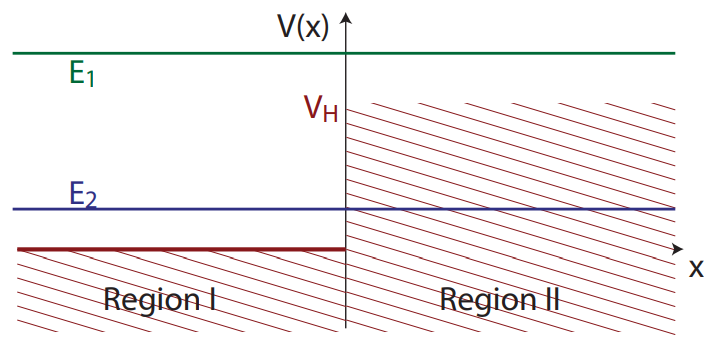
Let’s first consider the classical problem. The system is a rigid ball with total energy E given by the sum of the kinetic and potential energy. If we keep the total energy fixed, the kinetic energies are different in the two regions:
TI=ETII=E−VH
If E > VH, the kinetic energy in region two is TII=p22m=E−VH, yielding simply a reduced velocity for the particle. If E < VH instead, we would obtain a negative TII kinetic energy. This is not an allowed solution, but it means that the particle cannot travel into Region II and it’s instead confined in Region I: The particle bounces off the potential barrier.
In quantum mechanics we need to solve the Schrödinger equation in order to find the wavefunction describing the particle at any position. The time-independent Schrödinger equation is
Hψ(x)=−ℏ2d22mdx2ψ(x)+V(x)ψ(x)=Eψ(x)→{−ℏ22md2ψ(x)dx2=Eψ(x) in Region I −ℏ22md2ψ(x)dx2=(E−VH)ψ(x) in Region II
The two cases differ because in Region II the energy difference ΔE=E−VH is either positive or negative.
Positive energy
Let’s first consider the case in which ΔE=E−VH>0. In both regions the particle behaves as a free particle with energy EI = E and EII = E − VH. We have already seen the solutions to such differential equation. These are:
ψI(x)=Aeikx+Be−ikx
ψII(x)=Ceik′x+De−ik′x
where ℏ2k22m=E and ℏ2k′22m=E−VH.
We already interpreted the function eikx as a wave traveling from left to right and e−ikx as a wave traveling from right to left. We then consider a case similar to the classical case, in which a ball was sent toward a barrier. Then the particle is initially described as a wave traveling from left to right in Region I. At the potential barrier the particle can either be reflected, giving rise to a wave traveling from right to left in Region I, or be transmitted, yielding a wave traveling from left to right in Region II. This solution is described by the equations above if we set D = 0, implying that there is no wave originating from the far right.
Since the wavefunction should describe a physical situation, we want it to be a continuous function and with continuous derivative. Thus we have to match the solution values and their derivatives at the boundary x = 0. This will give equations for the coefficients, allowing us to find the exact solution of the Schrödinger equation. This is a boundary conditions problem.
From
ψI(0)=ψII(0) and ψ′I(0)=ψ′II(0)
and D = 0 we obtain the conditions:
A+B=C,ik(A−B)=ik′C
with solutions
B=k−k′k+k′A,C=2kk+k′A
We can further find A by interpreting the wavefunction in terms of a flux of particles. We thus fix the incoming wave flux to be Γ which sets |A|=√mΓℏk (we can consider A to be a real, positive number for simplicity). Then we have:
B=k−k′k+k′√mΓℏk,C=2kk+k′√mΓℏk
We can also verify the following identity
k|A|2=k|B|2+k′|C|2
which follows from:
k|B|2+k′|C|2=|A|2(k+k′)2[k(k−k′)2+k′(2k)2]=k|A|2(k−k′)2+4k′k(k+k′)2
Let us multiply it by ℏ/m=:
ℏkm|A|2=ℏkm|B|2+ℏk′m|C|2
Recall the interpretation of ψ(x)=Aeikx as a wave giving a flux of particles |ψ(x)|2v=|A|2ℏkm. This relationship similarly holds for the flux in region II as well as for the reflected flux. Then we can interpret the equality above as an equality of particle flux:
The incoming flux Γ=ℏkm|A|2 is equal to the sum of the reflected ΓR=ℏkm|B|2 and transmitted ΓT=ℏkm|C|2 fluxes. The particle flux is conserved. We can then define the reflection and transmission coefficients as:
Γ=ΓR+ΓT=RΓ+TΓ
where
R=k|B|2k|A|2=(k−k′k+k′)2,T=k′|C|2k|A|2=(2kk+k′)2k′k
It’s then easy to see that T+R=1 and we can interpret the reflection and transmission coefficients as the reflection and transmission probability, respectively.
In line with the probabilistic nature of quantum mechanics, we see that the solution of the Schrödinger equation does not give us a precise location for the particle. Instead it describes the probability of finding the particle at any point in space. Given the wavefunction found above we can then calculate various quantity of interest, such as the probability of the particle having a given momentum, position and energy.
Negative Energy
Now we turn to the case where E < VH, so that ΔE<0.. In the classical case we saw that this implied the impossibility for the ball to be in region II. In quantum mechanics we cannot simply guess a solution based on our intuition, but we need again to solve the Schrödinger equation. The only difference is that now in region II we have ℏ2k′′22m=E−VH<0.
As quantum mechanics is defined in a complex space, this does not pose any problem (we can have negative kinetic energies even if the total energy is positive) and we can solve for k′′ simply finding an imaginary number k′′=iκ, κ=√2mℏ2(VH−E) (with κ real).
The solutions to the eigenvalue problem are similar to what already seen:
ψI(x)=Aeikx+Be−ikx
ψII(x)=Ceik′′x=Ce−κx,
where we took D = 0 as before.
Quantum mechanics allows the particle to enter the classical forbidden region, but the wavefunction becomes a vanishing exponential function. This means that even if the particle can indeed enter the forbidden region, it cannot go very far, the probability of finding the particle far away from the potential barrier (given by P(x>0)=|ψII(x)|2=|C|2e−2κx becomes smaller and smaller.
Again we match the function and its derivatives at the boundary to find the coefficients:
ψI(0)=ψII(0)→A+B=C
ψ′I(0)=ψ′II(0)→ik(A−B)=−κC
with solutions
B=k−iκk+iκA,C=2kk+iκA
The situation in terms of flux is instead quite different. We now have the equality: k|B|2=k|A|2:
k|B|2=k|k−iκk+iκ|2=kk2+κ2k2+κ2=k
In terms of flux, we can write this relationship as Γ=ΓR, which implies R = 1 and T = 0. Thus we have no transmission, just perfect reflection, although there is a penetration of the probability in the forbidden region. This can be called an evanescent transmitted wave.
Finite barrier
We now consider a different potential which creates a finite barrier of height VH between x = 0 and L. As depicted in Figure 3.2.2 this potential divides the space in 3 regions. Again we consider two cases, where the total energy of the particle is greater or smaller than VH. Classically, we consider a ball initially in Region I. Then in the case where
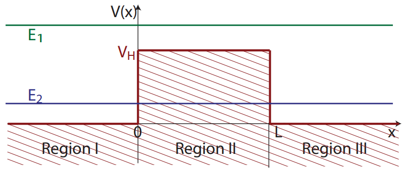
E > VH the ball can travel everywhere, in all the three regions, while for E < VH it is going to be confined in Region I, and we have perfect reflection. We will consider now the quantum mechanical case.
Positive kinetic energy
First we consider the case where ΔE=E−VH>0. The kinetic energies in the three regions are
Region I Region II Region III T=ℏ2k22m=ET=ℏ2k′22m=E−VHT=ℏ2k22m=E
And the wavefunction is
Region I Region II Region III Aeikx+Be−ikxCeik′x+De−ik′xEeikx
(again we put the term Fe−ikx=0 for physical reasons, in analogy with the classical case studied). The coefficients can be calculated by considering the boundary conditions.
In particular, we are interested in the probability of transmission of the beam through the barrier and into region III. The transmission coefficient is then the ratio of the outgoing flux in Region III to the incoming flux in Region I (both of these fluxes travel to the Right, so we label them by R):
T=k|ψRIII|2k|ψRI|2=k|E|2k|A|2=|E|2|A|2
while the reflection coefficient is the ratio of the reflected (from right to left, labeled L) and incoming (from left to right, labeled R) flux in Region I:
R=k|ψLI|2k|ψRI|2=k|B|2k|A|2=|B|2|A|2
We can solve explicitly the boundary conditions:
ψI(0)=ψII(0)ψII(L)=ψIII(L)
ψ′I(0)=ψ′II(0)ψ′II(L)=ψ′III(L)
and find the coefficients B, C, D, E (A is determined from the flux intensity Γ. From the full solution we can verify that T + R = 1, as it should be physically.
Obs. Notice that we could also have found a different solution, e.g. in which we set F≠0 and A = 0, corresponding to a particle originating from the right.
Negative Energy
In the case where ΔE=E−VH<0, in region II we expect as before an imaginary momentum. In fact we find
Region I Region II Region III k=√2mEℏ2k′=iκ,κ=√2m(VH−E)ℏ2k=√2mEℏ2
And the wavefunction is
Region I Region II Region III Aeikx+Be−ikxCe−κx+DeκxEeikx
The difference here is that a finite transmission through the barrier is possible and the transmission coefficient is not zero. Indeed, from the full solution of the boundary condition problem, we can find as in the previous case the coefficients T and R and we have T + R = 1.
There is thus a probability that the particle tunnels through the finite barrier and appears in Region III, then continuing to x → ∞.
Obs. Although we have been describing the situation in terms of wave traveling in one direction or the other, what we are describing here is not a time-dependent problem. There is no time-dependence at all in this problem (all the solutions are only a function of x, not of time). This is the same situation as stationary waves for example in a rope. The state of the system is not evolving. It is always (at any time) described by the same waves and thus at any time we will have the same outcomes and probability outcomes for any measurement.
Estimates and Scaling
Instead of solving exactly the problem for the second case, we try to make some estimates in the case there is a very small tunneling probability. In this case we have the following approximations for the coefficients A, B, C and D.
- Assuming T ≪ 1 we expect D ≈ 0 since if there is a very small probability for the particle to be in region III, the probability of coming back from it through the barrier must be even smaller (in other words, if D≠0 we would have an increasing probability to have a wave coming out of the barrier).
- Also, T ≪ 1 implies R ≈ 1. This means that B/A ≈ 1 or B ≈ A.
- Matching the wavefunction at x = 0, we have C = A + B ≈ 2A.
- Finally matching the wavefunction at x = L we obtain:
ψ(L)=Ce−κL=2Ae−κL=EeikL
We can then calculate the transmission probability T from T=k|ψRIII|2k|ψRI|2, with these assumptions. We obtain
T=k|E|2k|A|2=|E|2|A|2=4|A|2e−2κL|A|2→T=4e−2κL
Thus the transmission probability depends on the length of the potential barrier (the longer the barrier the less transmission we have, as it is intuitive) and on the coefficient κ. Notice that κ depends on the difference between the particle energy and the potential strength: If the particle energy is near the edge of the potential barrier (that is, ΔE ≈ 0) then κ ≈ 0 and there’s a high probability of tunneling. This case is however against our first assumptions of small tunneling (that’s why we obtain the unphysical result that T ≈ 4!!). The case we are considering is instead where the particle energy is small compared to the potential, so that κ is large, and the particle has a very low probability of tunneling through.