
3.3: Alpha Decay
- Page ID
- 25705
\( \newcommand{\vecs}[1]{\overset { \scriptstyle \rightharpoonup} {\mathbf{#1}} } \)
\( \newcommand{\vecd}[1]{\overset{-\!-\!\rightharpoonup}{\vphantom{a}\smash {#1}}} \)
\( \newcommand{\dsum}{\displaystyle\sum\limits} \)
\( \newcommand{\dint}{\displaystyle\int\limits} \)
\( \newcommand{\dlim}{\displaystyle\lim\limits} \)
\( \newcommand{\id}{\mathrm{id}}\) \( \newcommand{\Span}{\mathrm{span}}\)
( \newcommand{\kernel}{\mathrm{null}\,}\) \( \newcommand{\range}{\mathrm{range}\,}\)
\( \newcommand{\RealPart}{\mathrm{Re}}\) \( \newcommand{\ImaginaryPart}{\mathrm{Im}}\)
\( \newcommand{\Argument}{\mathrm{Arg}}\) \( \newcommand{\norm}[1]{\| #1 \|}\)
\( \newcommand{\inner}[2]{\langle #1, #2 \rangle}\)
\( \newcommand{\Span}{\mathrm{span}}\)
\( \newcommand{\id}{\mathrm{id}}\)
\( \newcommand{\Span}{\mathrm{span}}\)
\( \newcommand{\kernel}{\mathrm{null}\,}\)
\( \newcommand{\range}{\mathrm{range}\,}\)
\( \newcommand{\RealPart}{\mathrm{Re}}\)
\( \newcommand{\ImaginaryPart}{\mathrm{Im}}\)
\( \newcommand{\Argument}{\mathrm{Arg}}\)
\( \newcommand{\norm}[1]{\| #1 \|}\)
\( \newcommand{\inner}[2]{\langle #1, #2 \rangle}\)
\( \newcommand{\Span}{\mathrm{span}}\) \( \newcommand{\AA}{\unicode[.8,0]{x212B}}\)
\( \newcommand{\vectorA}[1]{\vec{#1}} % arrow\)
\( \newcommand{\vectorAt}[1]{\vec{\text{#1}}} % arrow\)
\( \newcommand{\vectorB}[1]{\overset { \scriptstyle \rightharpoonup} {\mathbf{#1}} } \)
\( \newcommand{\vectorC}[1]{\textbf{#1}} \)
\( \newcommand{\vectorD}[1]{\overrightarrow{#1}} \)
\( \newcommand{\vectorDt}[1]{\overrightarrow{\text{#1}}} \)
\( \newcommand{\vectE}[1]{\overset{-\!-\!\rightharpoonup}{\vphantom{a}\smash{\mathbf {#1}}}} \)
\( \newcommand{\vecs}[1]{\overset { \scriptstyle \rightharpoonup} {\mathbf{#1}} } \)
\(\newcommand{\longvect}{\overrightarrow}\)
\( \newcommand{\vecd}[1]{\overset{-\!-\!\rightharpoonup}{\vphantom{a}\smash {#1}}} \)
\(\newcommand{\avec}{\mathbf a}\) \(\newcommand{\bvec}{\mathbf b}\) \(\newcommand{\cvec}{\mathbf c}\) \(\newcommand{\dvec}{\mathbf d}\) \(\newcommand{\dtil}{\widetilde{\mathbf d}}\) \(\newcommand{\evec}{\mathbf e}\) \(\newcommand{\fvec}{\mathbf f}\) \(\newcommand{\nvec}{\mathbf n}\) \(\newcommand{\pvec}{\mathbf p}\) \(\newcommand{\qvec}{\mathbf q}\) \(\newcommand{\svec}{\mathbf s}\) \(\newcommand{\tvec}{\mathbf t}\) \(\newcommand{\uvec}{\mathbf u}\) \(\newcommand{\vvec}{\mathbf v}\) \(\newcommand{\wvec}{\mathbf w}\) \(\newcommand{\xvec}{\mathbf x}\) \(\newcommand{\yvec}{\mathbf y}\) \(\newcommand{\zvec}{\mathbf z}\) \(\newcommand{\rvec}{\mathbf r}\) \(\newcommand{\mvec}{\mathbf m}\) \(\newcommand{\zerovec}{\mathbf 0}\) \(\newcommand{\onevec}{\mathbf 1}\) \(\newcommand{\real}{\mathbb R}\) \(\newcommand{\twovec}[2]{\left[\begin{array}{r}#1 \\ #2 \end{array}\right]}\) \(\newcommand{\ctwovec}[2]{\left[\begin{array}{c}#1 \\ #2 \end{array}\right]}\) \(\newcommand{\threevec}[3]{\left[\begin{array}{r}#1 \\ #2 \\ #3 \end{array}\right]}\) \(\newcommand{\cthreevec}[3]{\left[\begin{array}{c}#1 \\ #2 \\ #3 \end{array}\right]}\) \(\newcommand{\fourvec}[4]{\left[\begin{array}{r}#1 \\ #2 \\ #3 \\ #4 \end{array}\right]}\) \(\newcommand{\cfourvec}[4]{\left[\begin{array}{c}#1 \\ #2 \\ #3 \\ #4 \end{array}\right]}\) \(\newcommand{\fivevec}[5]{\left[\begin{array}{r}#1 \\ #2 \\ #3 \\ #4 \\ #5 \\ \end{array}\right]}\) \(\newcommand{\cfivevec}[5]{\left[\begin{array}{c}#1 \\ #2 \\ #3 \\ #4 \\ #5 \\ \end{array}\right]}\) \(\newcommand{\mattwo}[4]{\left[\begin{array}{rr}#1 \amp #2 \\ #3 \amp #4 \\ \end{array}\right]}\) \(\newcommand{\laspan}[1]{\text{Span}\{#1\}}\) \(\newcommand{\bcal}{\cal B}\) \(\newcommand{\ccal}{\cal C}\) \(\newcommand{\scal}{\cal S}\) \(\newcommand{\wcal}{\cal W}\) \(\newcommand{\ecal}{\cal E}\) \(\newcommand{\coords}[2]{\left\{#1\right\}_{#2}}\) \(\newcommand{\gray}[1]{\color{gray}{#1}}\) \(\newcommand{\lgray}[1]{\color{lightgray}{#1}}\) \(\newcommand{\rank}{\operatorname{rank}}\) \(\newcommand{\row}{\text{Row}}\) \(\newcommand{\col}{\text{Col}}\) \(\renewcommand{\row}{\text{Row}}\) \(\newcommand{\nul}{\text{Nul}}\) \(\newcommand{\var}{\text{Var}}\) \(\newcommand{\corr}{\text{corr}}\) \(\newcommand{\len}[1]{\left|#1\right|}\) \(\newcommand{\bbar}{\overline{\bvec}}\) \(\newcommand{\bhat}{\widehat{\bvec}}\) \(\newcommand{\bperp}{\bvec^\perp}\) \(\newcommand{\xhat}{\widehat{\xvec}}\) \(\newcommand{\vhat}{\widehat{\vvec}}\) \(\newcommand{\uhat}{\widehat{\uvec}}\) \(\newcommand{\what}{\widehat{\wvec}}\) \(\newcommand{\Sighat}{\widehat{\Sigma}}\) \(\newcommand{\lt}{<}\) \(\newcommand{\gt}{>}\) \(\newcommand{\amp}{&}\) \(\definecolor{fillinmathshade}{gray}{0.9}\)If we go back to the binding energy per mass number plot (\(B/A\) vs. \(A\)) we see that there is a bump (a peak) for \(A ∼ 60 − 100\). This means that there is a corresponding minimum (or energy optimum) around these numbers. Then the heavier nuclei will want to decay toward this lighter nuclides, by shedding some protons and neutrons. More specifically, the decrease in binding energy at high \(A\) is due to Coulomb repulsion. Coulomb repulsion grows in fact as \(Z^2\), much faster than the nuclear force which is proportional to \(A\).
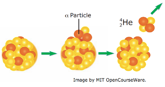
This could be thought as a similar process to what happens in the fission process: from a parent nuclide, two daughter nuclides are created. In the \(\alpha\) decay we have specifically:
\[\ce{_{Z}^{A} X_N -> _{Z-2}^{A-4} X_{N-2}^{\prime}} + \alpha \nonumber\]
where \(\alpha\) is the nucleus of \(\mathrm{He}-4:{ }_{2}^{4} \mathrm{He}_{2}\).
The \(\alpha\) decay should be competing with other processes, such as the fission into equal daughter nuclides, or into pairs including 12C or 16O that have larger B/A then \(\alpha\). However \(\alpha\) decay is usually favored. In order to understand this, we start by looking at the energetic of the decay, but we will need to study the quantum origin of the decay to arrive at a full explanation.
Energetics
In analyzing a radioactive decay (or any nuclear reaction) an important quantity is \(Q\), the net energy released in the decay: \(Q=\left(m_{X}-m_{X^{\prime}}-m_{\alpha}\right) c^{2}\). This is also equal to the total kinetic energy of the fragments, here \(Q=T_{X^{\prime}}+T_{\alpha} \) (here assuming that the parent nuclide is at rest).
When \(Q\) > 0 energy is released in the nuclear reaction, while for \(Q\) < 0 we need to provide energy to make the reaction happen. As in chemistry, we expect the first reaction to be a spontaneous reaction, while the second one does not happen in nature without intervention. (The first reaction is exo-energetic the second endo-energetic). Notice that it’s no coincidence that it’s called \(Q\). In practice given some reagents and products, \(Q\) give the quality of the reaction, i.e. how energetically favorable, hence probable, it is. For example in the alpha-decay \( \log \left(t_{1 / 2}\right) \propto \frac{1}{\sqrt{Q_{\alpha}}}\), which is the Geiger-Nuttall rule (1928).
The alpha particle carries away most of the kinetic energy (since it is much lighter) and by measuring this kinetic energy experimentally it is possible to know the masses of unstable nuclides.
We can calculate \(Q\) using the SEMF. Then:
\[Q_{\alpha}=B\left(\begin{array}{c}
A-4 \\
Z-2
\end{array} X_{N-2}^{\prime}\right)+B\left({ }^{4} H e\right)-B\left({ }_{Z}^{A} X_{N}\right)=B(A-4, Z-2)-B(A, Z)+B\left({ }^{4} H e\right) \nonumber\]
We can approximate the finite difference with the relevant gradient:
\[\begin{align}
Q_{\alpha} &=[B(A-4, Z-2)-B(A, Z-2)]+[B(A, Z-2)-B(A, Z)]+B\left({ }^{4} H e\right) \\[4pt] &\approx -4 \frac{\partial B}{\partial A}-2 \frac{\partial B}{\partial Z}+B\left({ }^{4} H e\right) \\[4pt] &=28.3-4 a_{v}+\frac{8}{3} a_{s} A^{-1 / 3}+4 a_{c}\left(1-\frac{Z}{3 A}\right)\left(\frac{Z}{A^{1 / 3}}\right)-4 a_{s y m}\left(1-\frac{2 Z}{A}+3 a_{p} A^{-7 / 4}\right)^{2} \end{align}\]
Since we are looking at heavy nuclei, we know that \(Z ≈ 0.41A\) (instead of \(Z ≈ A/2\)) and we obtain
\[Q_{\alpha} \approx-36.68+44.9 A^{-1 / 3}+1.02 A^{2 / 3}, \nonumber\]
where the second term comes from the surface contribution and the last term is the Coulomb term (we neglect the pairing term, since a priori we do not know if \(a_{p}\) is zero or not).
Then, the Coulomb term, although small, makes \(Q\) increase at large A. We find that \(Q \geq 0\) for \(A \gtrsim 150\), and it is \(Q\) ≈ 6MeV for A = 200. Although \(Q\) > 0, we find experimentally that \(\alpha\) decay only arise for \(A \geq 200\).
Further, take for example Francium-200 (\({ }_{87}^{200} \mathrm{Fr}_{113}\)). If we calculate \( Q_{\alpha}\) from the experimentally found mass differences we obtain \(Q_{\alpha} \approx 7.6 \mathrm{MeV}\) (the product is 196At). We can do the same calculation for the hypothetical decay into a 12C and remaining fragment (\({}_{81}^{188} \mathrm{TI}_{ \ 107}\)):
\[Q_{12} C=c^{2}\left[m\left(\begin{array}{c}
A \\
Z
\end{array} X_{N}\right)-m\left(\begin{array}{c}
A-12 \\
Z-6
\end{array} X_{N-6}^{\prime}\right)-m\left({ }^{12} C\right)\right] \approx 28 M e V \nonumber\]
Thus this second reaction seems to be more energetic, hence more favorable than the alpha-decay, yet it does not occur (some decays involving C-12 have been observed, but their branching ratios are much smaller).
Thus, looking only at the energetic of the decay does not explain some questions that surround the alpha decay:
- Why there’s no 12C-decay? (or to some of this tightly bound nuclides, e.g O-16 etc.)
- Why there’s no spontaneous fission into equal daughters?
- Why there’s alpha decay only for \(A \geq 200 \)?
- What is the explanation of Geiger-Nuttall rule? \(\log t_{1 / 2} \propto \frac{1}{\sqrt{Q_{\alpha}}}\)
Quantum mechanics description of alpha decay
We will use a semi-classical model (that is, combining quantum mechanics with classical physics) to answer the questions above.
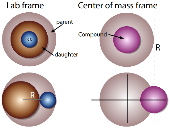
In order to study the quantum mechanical process underlying alpha decay, we consider the interaction between the daughter nuclide and the alpha particle. Just prior to separation, we can consider this pair to be already present inside the parent nuclide, in a bound state. We will describe this pair of particles in their center of mass coordinate frames: thus we are interested in the relative motion (and kinetic energy) of the two particles. As often done in these situations, we can describe the relative motion of two particles as the motion of a single particle of reduced mass \(\mu=\frac{m_{\alpha} m^{\prime}}{m_{\alpha}+m^{\prime}}\) (where m' is the mass of the daughter nuclide).
Consider for example the reaction \({ }^{238} \mathrm{U} \rightarrow{ }^{234} \mathrm{Th}+\alpha\). What is the interaction between the Th and alpha particle in the bound state?
- At short distance we have the nuclear force binding the 238U.
- At long distances, the coulomb interaction predominates
The nuclear force is a very strong, attractive force, while the Coulomb force among protons is repulsive and will tend to expel the alpha particle.
Since the final state is known to have an energy \( Q_{\alpha}=4.3 \ \mathrm{MeV}\), we will take this energy to be as well the initial energy of the two particles in the potential well (we assume that \(Q_{\alpha}=E \) since \(Q\) is the kinetic energy while the potential energy is zero). The size of the potential well can be calculated as the sum of the daughter nuclide (234Th) and alpha radii:
\[R=R^{\prime}+R_{\alpha}=R_{0}\left((234)^{1 / 3}+4^{1 / 3}\right)=9.3 \mathrm{fm} \nonumber\]
On the other side, the Coulomb energy at this separation is \(V_{C o u l}=e^{2} Z^{\prime} Z_{\alpha} / R=28 M e V \gg Q_{\alpha}\) (here Z' = Z − 2 ). Then, the particles are inside a well, with a high barrier (as \(V_{\text {Coul }} \gg Q \)) but there is some probability of tunneling, since Q > 0 and the state is not stably bound.
Thus, if the parent nuclide, \( {}^{238} \mathrm{U}\), was really composed of an alpha-particle and of the daughter nuclide, \( {}^{234} \mathrm{Th}\), then with some probability the system would be in a bound state and with some probability in a decayed state, with the alpha particle outside the potential barrier. This last probability can be calculated from the tunneling probability PT we studied in the previous section, given by the amplitude square of the wavefunction outside the barrier, \(P_{T}=\left|\psi\left(R_{\text {out}}\right)\right|^{2}\).
How do we relate this probability to the decay rate?
We need to multiply the probability of tunneling PT by the frequency \(f\) at which \( {}^{238} \mathrm{U}\) could actually be found as being in two fragments \({ }^{234} \mathrm{Th}+\alpha \) (although still bound together inside the potential barrier). The decay rate is then given by \(\lambda_{\alpha}=f P_{T}\).
To estimate the frequency \(f\), we equate it with the frequency at which the compound particle in the center of mass frame is at the well boundary: \(f=v_{i n} / R\), where \(v_{i n} \) is the velocity of the particles when they are inside the well (see cartoon in Figure \(\PageIndex{3}\)). We have \(\frac{1}{2} m v_{i n}^{2}=Q_{\alpha}+V_{0} \approx 40 \mathrm{MeV}\), from which we have \(v_{i n} \approx 4 \times 10^{22} \mathrm{fm} / \mathrm{s}\). Then the frequency is \(f \approx 4.3 \times 10^{21}\).
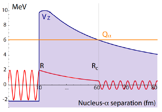
The probability of tunneling is given by the amplitude square of the wavefunction just outside the barrier, \(P_{T}=\left|\psi\left(R_{c}\right)\right|^{2}\), where Rc is the coordinate at which \(V_{\text {Coul }}\left(R_{c}\right)=Q_{\alpha}\), such that the particle has again a positive kinetic energy:
\[R_{c}=\frac{e^{2} Z_{\alpha} Z^{\prime}}{Q_{\alpha}} \approx 63 \mathrm{fm} \nonumber\]
Recall that in the case of a square barrier, we expressed the wavefunction inside a barrier (in the classically forbidden region) as a plane wave with imaginary momentum, hence a decaying exponential \( \psi_{i n}(r) \sim e^{-\kappa r}\). What is the relevant momentum \(\hbar \kappa \) here? Since the potential is no longer a square barrier, we expect the momentum (and kinetic energy) to be a function of position.
The total energy is given by \(E=Q_{\alpha} \) and is the sum of the potential (Coulomb) and kinetic energy. As we’ve seen that the Coulomb energy is higher than \(Q\), we know that the kinetic energy is negative:
\[Q_{\alpha}=T+V_{C o u l}=\frac{\hbar^{2} k^{2}}{2 \mu}+\frac{Z_{\alpha} Z^{\prime} e^{2}}{r} \nonumber\]
with µ the reduced mass
\[\mu=\frac{m_{\alpha} m^{\prime}}{m_{\alpha}+m^{\prime}} \nonumber\]
and \(k^{2}=-\kappa^{2} (with \( \kappa \in R\)). This equation is valid at any position inside the barrier:
\[\kappa(r)=\sqrt{\frac{2 \mu}{\hbar^{2}}\left[V_{C o u l}(r)-Q_{\alpha}\right]}=\sqrt{\frac{2 \mu}{\hbar^{2}}\left(\frac{Z_{\alpha} Z^{\prime} e^{2}}{r}-Q_{\alpha}\right)} \nonumber\]
If we were to consider a small slice of the barrier, from \(r\) to \(r + dr\), then the probability to pass through this barrier would be \(d P_{T}(r)=e^{-2 \kappa(r) d r}\). If we divide then the total barrier range into small slices, the final probability is the product of the probabilities \(d P_{T}^{k}\) of passing through all of the slices. Then \(\log \left(P_{T}\right)=\sum_{k} \log \left(d P_{T}^{k}\right)\) and taking the continuous limit \(\log \left(P_{T}\right)=\int_{R}^{R_{c}} \log \left[d P_{T}(r)\right]=-2 \int_{R}^{R_{c}} \kappa(r) d r\).
Finally the probability of tunneling is given by \(P_{T}=e^{-2 G} \), where G is calculated from the integral
\[G=\int_{R}^{R_{C}} d r \kappa(r)=\int_{R}^{R_{C}} d r \sqrt{\frac{2 \mu}{\hbar^{2}}\left(\frac{Z_{\alpha} Z^{\prime} e^{2}}{r}-Q_{\alpha}\right)} \nonumber\]
We can solve the integral analytically, by letting \( r=R_{c} y=y \frac{Z_{\alpha} Z^{\prime} e^{2}}{Q_{\alpha}}\), then
\[G=\frac{Z_{\alpha} Z_{0} e^{2}}{\hbar c} \sqrt{\frac{2 \mu c^{2}}{Q_{\alpha}}} \int_{R / R_{C}}^{1} d y \sqrt{\frac{1}{y}-1} \nonumber\]
which yields
\[G=\frac{Z_{\alpha} Z^{\prime} e^{2}}{\hbar c} \sqrt{\frac{2 \mu c^{2}}{Q_{\alpha}}}\left[\arccos \left(\sqrt{\frac{R}{R_{c}}}\right)-\sqrt{\frac{R}{R_{c}}} \sqrt{1-\frac{R}{R_{c}}}\right]=\frac{Z_{\alpha} Z^{\prime} e^{2}}{\hbar c} \sqrt{\frac{2 \mu c^{2}}{Q_{\alpha}}} \frac{\pi}{2} g\left(\sqrt{\frac{R}{R_{c}}}\right) \nonumber\]
where to simplify the notation we used the function
\[g(x)=\frac{2}{\pi}\left(\arccos (x)-x \sqrt{1-x^{2}}\right) . \nonumber\]
Finally the decay rate is given by
\[\boxed{\lambda_{\alpha}=\frac{v_{i n}}{R} e^{-2 G}} \nonumber\]
where G is the so-called Gamow factor.
In order to get some insight on the behavior of \(G\) we consider the approximation R ≪ Rc:
\[G=\frac{1}{2} \sqrt{\frac{E_{G}}{Q_{\alpha}}} g\left(\sqrt{\frac{R}{R_{c}}}\right) \approx \frac{1}{2} \sqrt{\frac{E_{G}}{Q_{\alpha}}}\left[1-\frac{4}{\pi} \sqrt{\frac{R}{R_{c}}}\right] \nonumber\]
where EG is the Gamow energy:
\[\boxed{E_{G}=\left(\frac{2 \pi Z_{\alpha} Z e^{2}}{\hbar c}\right)^{2} \frac{\mu c^{2}}{2}} \nonumber\]
For example for the \({ }^{238} \mathrm{U}\) decay studied EG = 122, 000MeV (huge!) so that \( \sqrt{E_{G} / Q_{\alpha}}=171\) while \(g\left(\sqrt{\frac{R}{R_{c}}}\right) \approx 0.518\). The exponent is thus a large number, giving a very low tunneling probabily: \(e^{-2 G}=e^{-89}=4 \times 10^{-39}\). Then, \(\lambda_{\alpha}=1.6 \times 10^{-17} \mathrm{~s}\) or \(t_{1 / 2}=4.5 \times 10^{9}\) years, close to what observed.
These results finally give an answer to the questions we had regarding alpha decay. The decay probability has a very strong dependence on not only \(Q_{\alpha} \) but also on Z1Z2 (where Zi are the number of protons in the two daughters). This leads to the following observations:
- Other types of decay are less likely, because the Coulomb energy would increase considerably, thus the barrier becomes too high to be overcome.
- The same is true for spontaneous fission, despite the fact that \(Q\) is much higher (∼ 200MeV).
- We thus find that alpha decay is the optimal mechanism. Still, it can happen only for A ≥ 200 exactly because otherwise the tunneling probability is very small.
- The Geiger-Nuttall law is a direct consequence of the quantum tunneling theory. Also, the large variations of the decay rates with \(Q\) are a consequence of the exponential dependence on \(Q\).
A final word of caution about the model: the semi-classical model used to describe the alpha decay gives quite accurate predictions of the decay rates over many order of magnitudes. However it is not to be taken as an indication that the parent nucleus is really already containing an alpha particle and a daughter nucleus (only, it behaves as if it were, as long as we calculate the alpha decay rates).