4.3: Solutions to the Schrödinger Equation in 3D

We now go back to the Schrödinger equation in spherical coordinates and we consider the angular and radial equation separately to find the energy eigenvalues and eigenfunctions.

Angular Equation

The angular equation was found to be:

\[\frac{1}{\sin \vartheta} \frac{\partial}{\partial \vartheta}\left(\sin \vartheta \frac{\partial Y_{l}^{m}(\vartheta, \varphi)}{\partial \vartheta}\right)+\frac{1}{\sin ^{2} \vartheta} \frac{\partial^{2} Y_{l}^{m}(\vartheta, \varphi)}{\partial \varphi^{2}}=-l(l+1) Y_{l}^{m}(\vartheta, \varphi) \nonumber\]

Notice that this equation does not depend at all on the potential, thus it will be common to all problems with an isotropic potential.

We can solve the equation by using again separation of variables: \(Y(\vartheta, \varphi)=\Theta(\vartheta) \Phi(\varphi)\). By multiplying both sides of the equation by \(\sin ^{2}(\vartheta) / Y(\vartheta, \varphi)\) we obtain:

\[\frac{1}{\Theta(\vartheta)}\left[\sin \vartheta \frac{d}{d \vartheta}\left(\sin \vartheta \frac{d \Theta}{d \vartheta}\right)\right]+l(l+1) \sin ^{2} \vartheta=-\frac{1}{\Phi(\varphi)} \frac{d^{2} \Phi}{d \varphi^{2}} \nonumber\]

As usual we separate the two equations in the different variables and introduce a constant C = m²:

\[\frac{d^{2} \Phi}{d \varphi^{2}}=-m^{2} \Phi(\varphi) \nonumber\]

\[\sin \vartheta \frac{d}{d \vartheta}\left(\sin \vartheta \frac{d \Theta}{d \vartheta}\right)=\left[m^{2}-l(l+1) \sin ^{2} \vartheta\right] \Theta(\vartheta) \nonumber\]

The first equation is easily solved to give \(\Phi(\varphi)=e^{i m \varphi}\) with \(m=0,\pm 1,\pm 2, \ldots\) since we need to impose the periodicity of \(\Phi\), such that \(\Phi(\varphi+2 \pi)=\Phi(\varphi)\).

The solutions to the second equations are associated Legendre Polynomials: \(\Theta(\vartheta)=A P_{l}^{m}(\cos \vartheta)\), the first few of l which are in table 1. Notice that, as previously found when solving for the eigenvalues of the angular momentum, we have that \(m = −l, −l + 1, . . . , l\), with \(l\) = 0, 1, . . . .

Table \(\PageIndex{1}\): Legendre Polynomials

The normalized angular eigenfunctions are then Spherical Harmonic functions, given by the normalized Legendre polynomial times the solution to the equation in \(\varphi\) (see also Table 2)

\[Y_{l}^{m}(\vartheta, \varphi)=\sqrt{\frac{(2 l+1)}{4 \pi} \frac{(l-m) !}{(l+m) !}} P_{l}^{m}(\cos \vartheta) e^{i m \varphi} \nonumber\]

As we expect from eigenfunctions, the Spherical Harmonics are orthogonal:

\[\int_{4 \pi} d \Omega Y_{l}^{m}(\vartheta, \varphi) Y_{l^{\prime}}^{m^{\prime}}(\vartheta, \varphi)=\delta_{l, l^{\prime}} \delta_{m, m^{\prime}} \nonumber\]

The radial equation

We now turn to the radial equation:

\[\frac{d}{d r}\left(r^{2} \frac{d R(r)}{d r}\right)-\frac{2 m r^{2}}{\hbar^{2}}(V-E)=l(l+1) R(r) \nonumber\]

Table \(\PageIndex{2}\): Spherical Harmonics

To simplify the solution, we introduce a different function \(u(r)=r R(r)\). Then the equation reduces to:

\[-\frac{\hbar^{2}}{2 m} \frac{d^{2} u}{d r^{2}}+\left[V+\frac{\hbar^{2}}{2 m} \frac{l(l+1)}{r^{2}}\right] u(r)=E u(r) \nonumber\]

This equation is very similar to the Schrödinger equation in 1D if we define an effective potential \(V^{\prime}(r)=V(r)+\frac{\hbar^{2}}{2 m} \frac{l(l+1)}{r^{2}}\). The second term in this effective potential is called the centrifugal term.

Solutions can be found for some forms of the potential V (\(r\)), by first calculating the equation solutions \(u_{n, l}(r)\), then finding \(R_{n, l}(r)=u_{n, l}(r) / r\) and finally the wavefunction

\[\Psi_{n, l, m}(r, \vartheta, \varphi)=R_{n, l}(r) Y_{l}^{m}(\vartheta, \varphi). \nonumber\]

Notice that we need 3 quantum numbers (n, l, m) to define the eigenfunctions of the Hamiltonian in 3D.

For example we can have a simple spherical well: V (\(r\)) = 0 for \(r<r_{0}\) and \(V(r)=V_{0}\) otherwise. In the case of \(l\) = 0, this is the same equation as for the square well in 1D. Notice however that since the boundary conditions need to be such that R(\(r\)) is finite for all \(r\), we need to impose that \(u(r=0)=0\), hence only the odd solutions are acceptable (as we had anticipated). For \(l\) > 0 we can find solutions in terms of Bessel functions.

Two other important examples of potential are the harmonic oscillator potential \(V(r)=V_{0} \frac{r^{2}}{r_{0}^{2}}-V_{0}\) (which is an approximation for any potential close to its minimum) and the Coulomb potential \(V(r)=-\frac{e^{2}}{4 \pi \epsilon_{0}} \frac{1}{r}\), which describes the atomic potential and in particular the Hydrogen atom.

The Hydrogen atom

We want to solve the radial equation for the Coulomb potential, or at least find the eigenvalues of the equation. Notice we are looking for bound states, thus the total energy is negative E < 0. Then we define the real quantity \(\kappa=\sqrt{\frac{-2 m E}{\hbar^{2}}}\), and the quantities⁸:

\[\text { Bohr radius: } a_{0}=\frac{4 \pi \epsilon_{0} \hbar^{2}}{m_{e} e^{2}}, \qquad \text { Rydberg constant: } \quad \mathbb{R}=\frac{\hbar^{2}}{2 m a_{0}^{2}} \nonumber\]

and \(\lambda^{2}=\frac{\mathbb{R}}{|E|}\). The values of the two constants are \(a_{0}=5.29 \times 10^{-11} \mathrm{~m}\) and \(\mathbb{R}=13.6 \mathrm{eV}\) (thus \(\lambda\) is a dimensionless parameter). The Bohr radius gives the distance at which the kinetic energy of an electron (classically) orbiting around the nucleus equals the Coulomb interaction: \(\frac{1}{2} m_{e} v^{2}=\frac{1}{4 \pi \epsilon_{0}} \frac{e^{2}}{r}\). In the semi-classical Bohr model, the angular momentum \(L=m_{e} v r\) is quantized, with lowest value \(L=\hbar\), then by inserting in the equation above, we find \(r=a_{0}\). We will see that the Rydberg energy gives instead the minimum energy for the hydrogen.

We further apply a change of variable\(\rho=2 \kappa r\), and we rewrite the radial equation as:

\[\frac{d^{2} u}{d \rho^{2}}=\left[\frac{1}{4}-\frac{\lambda}{\rho}+\frac{l(l+1)}{\rho^{2}}\right] u(\rho) \nonumber\]

There are two limiting cases:

For \(\rho \rightarrow 0\), the equation reduces to \(\frac{d^{2} u}{d \rho^{2}}=\frac{l(l+1)}{\rho^{2}} u\), with solution \(u(\rho) \sim \rho^{l+1}\).

For \(\rho \rightarrow \infty\) we have \(\frac{d^{2} u}{d \rho^{2}}=\frac{u(\rho)}{4}\), giving \(u(\rho) \sim e^{-\rho / 2}\).

Note

8 Note that the definition of the Bohr radius is slightly different if the Coulomb potential is not expressed in SI units but in cgs units

A general solution can then be written as \(u(\rho)=e^{-\rho / 2} \rho^{l+1} S(\rho) \) (with S to be determined). We then expand \( S(\rho)\) in series as \( S(\rho)=\sum_{j=0}^{\infty} s_{j} \rho^{j}\) and try to find the coefficients \(s_{j} \). By inserting \( u(\rho)=e^{-\rho / 2} \rho^{l+1} \sum_{j=0}^{\infty} s_{j} \rho^{j}\) in the equation we have:

\[\left[\rho \frac{d^{2}}{d \rho^{2}}+(2 l+2-\rho) \frac{d}{d \rho}-(l+1-\lambda)\right] S(\rho)=0 \nonumber\]

From which we obtain:

\[\sum_{j}\left[\rho\left\{j(j+1) s_{j+1} \rho^{j-1}\right\}+(2 l+2-\rho)\left\{(j+1) s_{j+1} \rho^{j}\right\}-(l+1-\lambda)\left\{s_{j} \rho^{j}\right\}\right]=0 \nonumber\]

(where the terms in brackets correspond to the derivatives of \(S(\rho) \)). This equation defines a recursive equation for the coefficients \(s_{j}\):

\[s_{j+1}=\frac{j+l+1-\lambda}{j(j+1)+(2 l+2)(j+1)} s_{j} \nonumber\]

If we want the function \(u(\rho) \) to be well defined, we must impose that \(u(\rho) \rightarrow 0 \) for \( \rho \rightarrow \infty\). This imposes a maximum value for \(j, j_{\max } \), such that all the higher coefficients \({s}_{j}>j_{\max } \) are zero.

Then we have that \( j_{\max }+l+1-\lambda=0\). But this is an equation for \(\lambda \), which in turns determines the energy eigenvalue:

\[\lambda=j_{\max }+l+1. \nonumber\]

We then rename the parameter \( \lambda \) the principal quantum number \(n\) since it is an integer (as j and l are integers). Then the energy is given by \( E=-\frac{\mathbb{R}}{n^{2}} \) and the allowed energies are given by the famous Bohr formula:

\[\boxed{E_{n}=-\frac{1}{n^{2}} \frac{m_{e}}{2 \hbar^{2}}\left(\frac{e^{2}}{4 \pi \epsilon_{0}}\right)^{2}} \nonumber\]

Obs.

Note that the energy is only determined by the principal quantum number. What is the degeneracy of the\(n\)quantum number? We know that the full eigenfunction is specified by knowing the angular momentum L² and one of its components (e.g. \(L_{z} \)). From the equation above, \( n=j_{\max }+l+1\), we see that for each \(n, l\) can vary from \(l\) = 0 to \(l\) =\(n\)− 1. Then we also have 2\(l\) + 1 \(m\) values for each l (and 2 spin states for each m). Finally, the degeneracy is then given by

\[\sum_{l=0}^{n-1} 2(2 l+1)=2 n^{2} \nonumber\]

Atomic periodic structure

We calculated the energy levels for the Hydrogen atom. This will give us spectroscopy information about the excited states that we can excite using, for example, laser light. How can we use this information to infer the structure of the atoms?

A neutral atom, of atomic number Z, consists of a heavy nucleus, with electric charge Ze, surrounded by Z electrons (mass \(m\) and charge -e). The Hamiltonian for this system is

\[\mathcal{H}=\sum_{j=1}^{Z}\left[-\frac{\hbar^{2}}{2 m} \nabla_{j}^{2}-\frac{1}{4 \pi \epsilon_{0}} \frac{Z e^{2}}{r_{j}}\right]+\frac{1}{2} \frac{1}{4 \pi \epsilon_{0}} \sum_{j \neq k}^{Z} \frac{e^{2}}{\left|\vec{r}_{j}-\vec{r}_{k}\right|} \nonumber\]

The first term is simply the kinetic energy of each electron in the atom. The second term is the potential energy of the jth electron in the electric field created by the nucleus. Finally the last sum (which runs over all values of j and k except j = k) is the potential energy associated with the mutual repulsion of the electrons (the factor of 1/2 in front corrects for the fact that the summation counts each pair twice).

Given this Hamiltonian, we want to find the energy levels (and in particular the ground state, which will give us the stable atomic configuration). We then need to solve Schrödinger ’s equation. But what would an eigenstate of this equation now be?

Consider for example Helium, an atom with only two electrons. Neglecting for the moment spin, we can write the wavefunction as \( \Psi\left(\vec{r}_{1}, \vec{r}_{2}, t\right)\) (and stationary wavefunctions, \(\psi\left(\vec{r}_{1}, \vec{r}_{2}\right) \)), that is, we have a function of the spatial coordinates of both electrons. The physical interpretation of the wavefunction is a simple extension of the one-particle wavefunction: \( \left|\psi\left(\vec{r}_{1}, \vec{r}_{2}\right)\right|^{2} d^{3} \vec{r}_{1} d^{3} \vec{r}_{2}\) is the probability of finding contemporaneously the two electrons at the positions \( \vec{r}_{1}\) and \( \vec{r}_{2}\), respectively. The wavefunction must then be normalized as \(\int\left|\psi\left(\vec{r}_{1}, \vec{r}_{2}\right)\right|^{2} d^{3} \vec{r}_{1} d^{3} \vec{r}_{2}=1 \). The generalization to many electrons (or more generally to many particles) is then evident.

To determine the ground state of an atom we will then have to solve the Schrödinger equation

\[\mathcal{H} \psi\left(\vec{r}_{1}, \ldots, \vec{r}_{Z}\right)=E \psi\left(\vec{r}_{1}, \ldots, \vec{r}_{Z}\right) \nonumber \]

This equation has not been solved (yet) except for the case Z=1 of the Hydrogen atom we saw earlier. What we can do is to make a very crude approximation and ignore the Coulomb repulsion among electrons. Mathematically this simplifies tremendously the equation, since now we can simply use separation of variables to write many equations for each independent electron. Physically, this is often a good enough approximation because mutual repulsion of electron is not as strong as the attraction from all the protons. Then the Schrödinger equation becomes:

\[\sum_{j=1}^{Z}\left[-\frac{\hbar^{2}}{2 m} \nabla_{j}^{2}-\frac{1}{4 \pi \epsilon_{0}} \frac{Z e^{2}}{r_{j}}\right] \psi\left(\vec{r}_{1}, \ldots, \vec{r}_{Z}\right)=E \psi\left(\vec{r}_{1}, \ldots, \vec{r}_{Z}\right) \nonumber\]

and we can write \( \psi\left(\vec{r}_{1}, \ldots, \vec{r}_{Z}\right)=\psi\left(\vec{r}_{1}\right) \psi\left(\vec{r}_{2}\right) \ldots \psi\left(\vec{r}_{Z}\right)\)

Then, we can solve for each electron separately, as we did for the Hydrogen atom equation, and find for each electron the same level structure as for the Hydrogen, except that the since the potential energy is now \( \frac{1}{4 \pi \epsilon_{0}} \frac{Z e^{2}}{r_{j}}\) the electron energy (Bohr’s formula) is now multiplied by Z. The solutions to the time-independent Schrödinger equations are then the same eigenfunctions we found for the hydrogen atom, \(\psi\left(\vec{r}_{j}=\psi_{l m n}(r, \vartheta, \varphi)\right. \).

Thus if we ignore the mutual repulsion among electrons, the individual electrons occupy one-particle hydrogenic states (\(n, l, m\)), called orbitals, in the Coulomb potential of a nucleus with charge Ze.

There are 2\(n\)² hydrogenic wave functions (all with the same energy \(E_{n}\)) for a given value of \(n\). Looking at the Periodic Table we see this periodicity, with two elements in the\(n\)= 1 shell, 8 in the\(n\)= 2 shell, 18 in the third shell. Higher shells however are more influenced by the electron-electron repulsion that we ignored, thus simple considerations from this model are no longer valid.

However, we would expect instead the electrons in the atoms to occupy the state with lowest energy. The ground state would then be a situation were all the electron occupy their own ground state (\(n\) = 0, \(l\) = 0, \(m\) = 0). But is this correct? This is not what is observed in nature, otherwise all the atom would show the same chemical properties. So what happens?

To understand, we need to analyze the statistical properties of identical particles. But before that, we will intro­duce the solution for another central potential, the harmonic oscillator potential \(V(r)=V_{0} \frac{r^{2}}{r_{0}^{2}}-V_{0} \) (which is an approximation for any potential close to its minimum).

The Harmonic Oscillator Potential

The quantum h.o. is a model that describes systems with a characteristic energy spectrum, given by a ladder of evenly spaced energy levels. The energy difference between two consecutive levels is \(\Delta E\). The number of levels is infinite, but there must exist a minimum energy, since the energy must always be positive. Given this spectrum, we expect the Hamiltonian will have the form

\[\mathcal{H}|n\rangle=\left(n+\frac{1}{2}\right) \quad \omega|n\rangle, \nonumber\]

where each level in the ladder is identified by a number \(n\). The name of the model is due to the analogy with characteristics of classical h.o., which we will review first.

Classical harmonic oscillator and h.o. model

A classical h.o. is described by a potential energy \( V=\frac{1}{2} k x^{2}\) (the radial potential considered above, \(V(r)=V_{0} \frac{r^{2}}{r_{0}^{2}}-V_{0} \), has this form). If the system has a finite energy E, the motion is bound by two values \(\pm x_{0} \), such that \( V\left(x_{0}\right)=E\). The equation of motion is given by

\[\left\{\begin{array}{l} \frac{d x}{d t}=\frac{p(t)}{m}, \\ \frac{d p}{d t}=-k x \end{array} \rightarrow \quad m \frac{d^{2} x}{d x^{2}}=-k x\right., \nonumber\]

and the kinetic energy is of course

\[T=\frac{1}{2} m \dot{x}^{2}=\frac{p^{2}}{2 m}. \nonumber\]

The energy is constant since it is a conservative system, with no dissipation. Most of the time the particle is in the position \(x_{0}\) since there the velocity is zero, while at x = 0 the velocity is maximum.

The h.o. oscillator in QM is an important model that describes many different physical situations. It describes e.g. the electromagnetic field, vibrations of solid-state crystals and (a simplified model of) the nuclear potential. This is because any potential with a local minimum can be locally described by an h.o.. Provided that the energy is low enough (or x close to \(x_{0}\)), any potential can in fact be expanded in series, giving: \(V(x) \approx V\left(x_{0}\right)+b\left(x-x_{0}\right)^{2}+\ldots\) where \(b=\left.\frac{d^{2} V}{d x^{2}}\right|_{x_{0}}\).

It is easy to solve the equation of motion. Instead of just solving the usual equation, we follow a slightly different route. We define dimensionless variables,

\[P=\frac{p}{\sqrt{m \omega}}, \quad X=x \sqrt{m \omega} \nonumber\]

where we defined a parameter with units of frequency: \(\omega=\sqrt{k / m}\) and we introduce a complex classical variable (following Roy J. Glauber –Phys. Rev. 131, 2766–2788 (1963))

\[\alpha=\frac{1}{\sqrt{2}}(X+i P). \nonumber\]

The classical equations of motion for x and p define the evolution of the variable \(\alpha \):

\[\left\{\begin{array}{l}
\frac{d x}{d t}=\frac{p(t)}{m}, \\
\frac{d p}{d t}=-k x
\end{array} \quad \rightarrow \quad \frac{d \alpha}{d t}=-i \omega \alpha(t)\right. \nonumber\]

The evolution of \(\alpha\) is therefore just a rotation in its phase space: \(\alpha(t)=\alpha(0) e^{-i \omega t}\).

Since \(X=\sqrt{2} \operatorname{Re}(\alpha)\) and \(P=\sqrt{2} operatorname{Im}(\alpha), X\) and \(P\) oscillate, as usual in the classical case:

\[\begin{array}{l}
X=\frac{1}{\sqrt{2}}\left(\alpha_{0} e^{-i \omega t}+\alpha_{0}^{*} e^{i \omega t}\right) \\
P=\frac{-i}{\sqrt{2}}\left(\alpha_{0} e^{-i \omega t}-\alpha_{0}^{*} e^{i \omega t}\right)
\end{array} \nonumber\]

The classical energy, given by \( \omega / 2\left(X^{2}+P^{2}\right)=\omega \alpha_{0}^{2}\), is constant at all time.

Oscillator Hamiltonian: Position and momentum operators

Using the operators associated with position and momentum, the Hamiltonian of the quantum h.o. is written as:

\[\mathcal{H}=\frac{p^{2}}{2 m}+\frac{k x^{2}}{2}=\frac{p^{2}}{2 m}+\frac{1}{2} m \omega^{2} x^{2}. \nonumber\]

In terms of the dimensionless variables, P and X, the Hamiltonian is \( \mathcal{H}=\frac{\omega}{2}\left(X^{2}+P^{2}\right)\).

In analogy with the classical variable a(t) [and its complex conjugate a^∗(t), which simplified the equation of motion, we introduce two operators, a, a^†, hoping to simplify the eigenvalue equation (time-independent Schrödinger equation):

\[\begin{array}{l}
a=\frac{1}{\sqrt{2 \hbar}}(X+i P)=\frac{1}{\sqrt{2 \hbar}}\left(\sqrt{m \omega} x+\frac{i}{\sqrt{m \omega}} p\right) \\
a^{\dagger}=\frac{1}{\sqrt{2 \hbar}}(X-i P)=\frac{1}{\sqrt{2 \hbar}}\left(\sqrt{m \omega} x-\frac{i}{\sqrt{m \omega}} p\right),
\end{array} \nonumber\]

Also, we define the number operator as N = a^†a, with eigenvalues n and eigenfunctions \(|n\rangle\). The Hamiltonian can be written in terms of these operators. We substitute a, a^† at the place of X and P, yielding \(\mathcal{H}=\hbar \omega\left(a^{\dagger} a+\frac{1}{2}\right)=\hbar \omega\left(N+\frac{1}{2}\right)\) and the minimum energy \( \omega / 2\) is called the zero point energy.

The commutation properties are: \(\left[a, a^{\dagger}\right]=1\) and \([N, a]=-a,\left[N, a^{\dagger}\right]=a^{\dagger}\). Also we have:

\[\begin{array}{l}
x=\sqrt{\frac{\hbar}{2 m \omega}}\left(a^{\dagger}+a\right) \\
p=i \sqrt{\frac{m \omega \hbar}{2}}\left(a^{\dagger}-a\right)
\end{array} \nonumber\]

□ Prove the commutation relationships of the raising and lowering operators.

\[\left[a, a^{\dagger}\right]=\frac{1}{2}[X+i P, X-i P]=\frac{1}{2}([X,-i P]+[i P, X])=-\frac{i}{\hbar}[X, P]=-\frac{i}{\hbar}[x, p]=1 \nonumber\]

So we also have \(a a^{\dagger}=\left[a, a^{\dagger}\right]+a^{\dagger} a=1+a^{\dagger} a=1+N\).

\[[N, a]=\left[a^{\dagger} a, a\right]=\left[a^{\dagger}, a\right] a=-a \quad \text { and } \quad\left[N, a^{\dagger}\right]=\left[a^{\dagger} a, a^{\dagger}\right]=a^{\dagger}\left[a, a^{\dagger}\right]=a^{\dagger} \nonumber\]

□

From the commutation relationships we have:

\[a|n\rangle=[a, N]|n\rangle=a n|n\rangle-N a|n\rangle \rightarrow N(a|n\rangle)=(n-1)(a|n\rangle) , \nonumber\]

that is, \(a|n\rangle \) is also an eigenvector of the N operator, with eigenvalue (n − 1). Thus we confirm that this is the lowering operator: \(a|n\rangle=c_{n}|n-1\rangle\). Similarly, \( a^{\dagger}|n\rangle\) is an eigenvector of N with eigenvalue n + 1:

\[a^{\dagger}|n\rangle=\left[N, a^{\dagger}\right]|n\rangle=N a^{\dagger}|n\rangle-a^{\dagger} n|n\rangle \rightarrow N\left(a^{\dagger}|n\rangle\right)=(n+1)(a|n\rangle). \nonumber\]

We thus have \( a|n\rangle=c_{n}|n-1\rangle\) and \(a^{\dagger}|n\rangle=d_{n}|n+1\rangle \). What are the coefficients c_n, d_n?

Since

\[\langle n|N| n\rangle=\left\langle n\left|a^{\dagger} a\right| n\right\rangle=n \nonumber\]

and

\[\left\langle n\left|a^{\dagger} a\right| n\right\rangle=(\langle a n|)(a|n\rangle)=\langle n-1 \mid n-1\rangle c_{n}^{2}, \nonumber\]

we must have \(c_{n}=\sqrt{n} \). Analogously, since \( a a^{\dagger}=N+1\), as seen from the commutation relationship:

\[d_{n}^{2}\langle n+1 \mid n+1\rangle=\left\langle a^{\dagger} n \mid a^{\dagger} n\right\rangle=\left\langle n\left|a a^{\dagger}\right| n\right\rangle\langle n|(N+1)| n\rangle=n+1 \nonumber\]

So in the end we have :

\[\boxed{a|n\rangle=\sqrt{n}|n-1\rangle ; \quad a^{\dagger}|n\rangle=\sqrt{n+1}|n+1\rangle.} \nonumber\]

All the n eigenvalues of N have to be non-negative since \(n=\langle n|N| n\rangle=\left\langle\psi_{n_{1}} \mid \psi_{n_{1}}\right\rangle \geq 0\) (this follows from the properties of the inner product and the fact that \(\left|\psi_{n_{1}}\right\rangle=a|n\rangle \) is just a regular state vector). However, if we apply over and over the a (lowering) operator, we could arrive at negative numbers n: we therefore require that \(a|0\rangle=0 \) to truncate this process. The action of the raising operator a^† can then produce any eigenstate, starting from the 0 eigenstate:

\[|n\rangle=\frac{\left(a^{\dagger}\right)^{n}}{\sqrt{n !}}|0\rangle. \nonumber\]

The matrix representation of these operator in the \(|n\rangle \) basis (with infinite-dimensional matrices) is particularly simple, since \(\left\langle n|a| n^{\prime}\right\rangle=\delta_{n^{\prime}, n-1} \sqrt{n}\) and \( \left\langle n\left|a^{\dagger}\right| n^{\prime}\right\rangle=\delta_{n^{\prime}, n+1} \sqrt{n+1}\):

\[a=\left[\begin{array}{cccc}
0 & \sqrt{1} & 0 & \ldots \\
0 & 0 & \sqrt{2} & \ldots \\
0 & 0 & 0 & \ldots
\end{array}\right] \qquad a^{\dagger}=\left[\begin{array}{cccc}
0 & 0 & 0 & \ldots \\
\sqrt{1} & 0 & 0 & \ldots \\
0 & \sqrt{2} & 0 & \ldots
\end{array}\right] \nonumber\]

Position representation

Figure \(\PageIndex{1}\): Left: Harmonic oscillator wavefunction. Right: corresponding probability distribution function for n = 2 (blue) and n = 3 (Red, dotted). (Copyright; author via source)

We have now started from a (physical) description of the h.o. Hamiltonian and made a change of basis in order to arrive at a simple diagonal form of it. Now that we know its eigenkets, we would like to go back to a more intuitive picture of position and momentum. We thus want to express the eigenkets \(|n\rangle\) in terms of the position representation.

Figure \(\PageIndex{2}\): Left: Harmonic oscillator wavefunction. Right: corresponding probability distribution function for n = 40. In Red, the classical probability. (Copyright; author via source)

The position representation corresponds to expressing a state vector \(|\psi\rangle\) in the position basis: \(|\psi\rangle=\int d x\langle x \mid \psi\rangle|x\rangle=\int d x \psi(x)|x\rangle\) (where \(|x\rangle\) is the eigenstate of the position operator that is a continuous variable, hence the integral). This defines the wavefunction \( \psi(x)=\langle x \mid \psi\rangle\).

The wave function description in the x representation of the quantum h.o. can be found by starting with the ground state wavefunction. Since \(a|0\rangle=0\) we have \(\frac{1}{\sqrt{2 \hbar}}(X+i P)|0\rangle=\frac{1}{\sqrt{2 \hbar}}\left(\sqrt{m \omega} x+\frac{i p}{\sqrt{m \omega}}\right)|0\rangle=0\). In the x representation, given \(\psi_{0}(x)=\langle x \mid 0\rangle\)

\[\frac{1}{\sqrt{2 \hbar}}\left\langle x\left|\left(\sqrt{m \omega} x+\frac{i p}{\sqrt{m \omega}}\right)\right| 0\right\rangle=0 \quad \rightarrow \quad\left(m \omega x+\frac{d}{d x}\right) \psi_{0}(x)=0 \quad \rightarrow \quad \psi_{0}(x) \propto e^{-m \omega x^{2} / 2} \nonumber\]

The other eigenstates are built using Hermite Polynomials \( H_{n}(x)\), using the formula⁹ \(|n\rangle=\frac{\left(a^{\dagger}\right)^{n}}{\sqrt{n !}}|0\rangle\) to derive differential equations:

\[\psi_{n}(x)=\langle x \mid n\rangle=\frac{1}{\sqrt{n !} 2^{n}}\left[\sqrt{m \omega} x-\frac{1}{\sqrt{m \omega}} \frac{d}{d x}\right]^{n} \psi_{0}(x) \nonumber\]

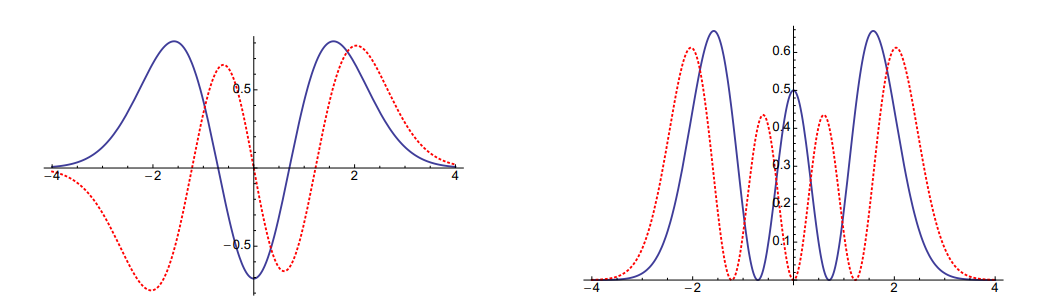
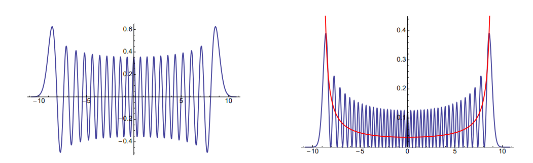
with solutions \(\psi_{n}(x)=\langle x \mid n\rangle=\frac{1}{\sqrt{2^{n} n !}} H_{n}(x) \psi_{0}(x)\). The n = 2 and n = 3 wavefunctions are plotted in the following figure, while the second figure displays the probability distribution function. Notice the different parity for even and odd number and the number of zeros of these functions. Classically, the probability that the oscillating particle is at a given value of x is simply the fraction of time that it spends there, which is inversely proportional to its velocity \(v(x)=x_{0} \omega \sqrt{1-\frac{x^{2}}{x_{0}^{2}}}\) at that position. For large n, the probability distribution becomes close to the classical one (see Fig. 4.3.2).

Note

9 For more details on Hermite Polynomials and their generator function, look on Cohen-Tannoudji. Online information from: Eric W. Weisstein. Hermite Polynomial. From MathWorld–A Wolfram Web Resource.