
7.1: Gamma Decay
- Page ID
- 25731

Gamma decay is the third type of radioactive decay. Unlike the two other types of decay, it does not involve a change in the element. It is just a simple decay from an excited to a lower (ground) state. In the process of course some energy is released that is carried away by a photon. Similar processes occur in atomic physics, however there the energy changes are usually much smaller, and photons that emerge are in the visible spectrum or x-rays.
The nuclear reaction describing gamma decay can be written as
\[{ }_{Z}^{A} X^{*} \rightarrow{ }_{Z}^{A} X+\gamma \nonumber\]
where ∗ indicates an excited state.
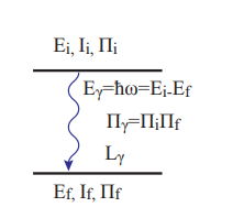
We have said that the photon carries aways some energy. It also carries away momentum, angular momentum and parity (but no mass or charge) and all these quantities need to be conserved. We can thus write an equation for the energy and momentum carried away by the gamma-photon.
From special relativity we know that the energy of the photon (a massless particle) is
\[E=\sqrt{m^{2} c^{4}+p^{2} c^{2}} \rightarrow \quad E=p c \nonumber\]
(while for massive particles in the non-relativistic limit \(v \ll c\) we have \(E \approx m c^{2}+\frac{p^{2}}{2 m}\).) In quantum mechanics we have seen that the momentum of a wave (and a photon is well described by a wave) is \(p=\hbar k\) with \(k\) the wave number. Then we have
\[\boxed{E=\hbar k c=\hbar \omega_{k}} \nonumber\]
This is the energy for photons which also defines the frequency \(\omega_{k}=k c\) (compare this to the energy for massive particles, \(E=\frac{\hbar^{2} k^{2}}{2 m}\)).
Gamma photons are particularly energetic because they derive from nuclear transitions (that have much higher energies than e.g. atomic transitions involving electronic levels). The energies involved range from \(E \sim .1 \div 10 \mathrm{MeV}\), giving \(k \sim 10^{-1} \div 10^{-3} \mathrm{fm}^{-1}\). Than the wavelengths are \(\lambda=\frac{2 \pi}{k} \sim 100 \div 10^{4} \mathrm{fm} \), much longer than the typical nuclear dimensions.
Gamma ray spectroscopy is a basic tool of nuclear physics, for its ease of observation (since it’s not absorbed in air), accurate energy determination and information on the spin and parity of the excited states. Also, it is the most important radiation used in nuclear medicine.
Classical Theory of Radiation
From the theory of electrodynamics it is known that an accelerating charge radiates. The power radiated is given by the integral of the energy flux (as given by the Poynting vector) over all solid angles. This gives the radiated power as:
\[\boxed{P=\frac{2}{3} \frac{e^{2}|a|^{2}}{c^{3}}} \nonumber\]
where \(a\) is the acceleration. This is the so-called Larmor formula for a non-relativistic accelerated charge.
As an important example we consider an electric dipole. An electric dipole can be considered as an oscillating charge, over a range \(r_{0} \), such that the electric dipole is given by \( d(t)=q r(t)\). Then the equation of motion is
\[r(t)=r_{0} \cos (\omega t) \nonumber\]
and the acceleration
\[a=\ddot{r}=-r_{0} \omega^{2} \cos (\omega t) \nonumber\]
Averaged over a period \(T=2 \pi / \omega\), this is
\[\left\langle a^{2}\right\rangle=\frac{\omega}{2 \pi} \int_{0}^{T} d t a(t)=\frac{1}{2} r_{0}^{2} \omega^{4} \nonumber\]
Finally we obtain the radiative power for an electric dipole:
\[P_{E 1}=\frac{1}{3} \frac{e^{2} \omega^{4}}{c^{3}}\left|\vec{r}_{0}\right|^{2} \nonumber\]
Electromagnetic Multipoles
In order to determine the classical e.m. radiation we need to evaluate the charge distribution that gives rise to it. The electrostatic potential of a charge distribution \(\rho_{e}(r)\) is given by the integral:
\[V(\vec{r})=\frac{1}{4 \pi \epsilon_{0}} \int_{V o l^{\prime}} \frac{\rho_{e}\left(\overrightarrow{r^{\prime}}\right)}{\left|\vec{r}-\overrightarrow{r^{\prime}}\right|} \nonumber\]
When treating radiation we are only interested in the potential outside the charge and we can assume the charge (e.g. a particle!) to be well localized (\(r^{\prime} \ll r\)). Then we can expand \(\frac{1}{\left|\vec{r}-\vec{r}^{\prime}\right|}\) in power series. First, we express explicitly the norm
\[\left|\vec{r}-\vec{r}^{\prime}\right|=\sqrt{r^{2}+r^{\prime 2}-2 r r^{\prime} \cos \vartheta}=r \sqrt{1+\left(\frac{r^{\prime}}{r}\right)^{2}-2 \frac{r^{\prime}}{r} \cos \vartheta}. \nonumber\]
We set
\[R=\frac{r^{\prime}}{r} \nonumber\]
and
\[\epsilon=R^{2}-2 R \cos \vartheta. \nonumber\]
This is a small quantity, given the assumption \(r^{\prime} \ll r\). Then we can expand:
\[\frac{1}{\left|\vec{r}-\vec{r}^{\prime}\right|}=\frac{1}{r} \frac{1}{\sqrt{1+\epsilon}}=\frac{1}{r}\left(1-\frac{1}{2} \epsilon+\frac{3}{8} \epsilon^{2}-\frac{5}{16} \epsilon^{3}+\ldots\right) \nonumber\]
Replacing \(\epsilon\) with its expression we have:
\[\begin{align*} \frac{1}{r} \frac{1}{\sqrt{1+\epsilon}} &=\frac{1}{r}\left(1-\frac{1}{2}\left(R^{2}-2 R \cos \vartheta\right)+\frac{3}{8}\left(R^{2}-2 R \cos \vartheta\right)^{2}-\frac{5}{16}\left(R^{2}-2 R \cos \vartheta\right)^{3}+\ldots\right) \\[4pt]
&=\frac{1}{r}\left(1+\left[-\frac{1}{2} R^{2}+R \cos \vartheta\right]+\left[\frac{3}{8} R^{4}-\frac{3}{2} R^{3} \cos \vartheta+\frac{3}{2} R^{2} \cos ^{2} \vartheta\right]+\left[-\frac{5 R^{6}}{16}+\frac{15}{8} R^{5} \cos (\vartheta)-\frac{15}{4} R^{4} \cos ^{2}(\vartheta)+\frac{5}{2} R^{3} \cos ^{3}(\vartheta)\right]+\ldots\right) \\[4pt]
&=\frac{1}{r}\left(1+R \cos \vartheta+R^{2}\left(\frac{3 \cos ^{2} \vartheta}{2}-\frac{1}{2}\right)+R^{3}\left(\frac{5 \cos ^{3}(\vartheta)}{2}-\frac{3 \cos (\vartheta)}{2}\right)+\ldots\right)
\end{align*} \]
We recognized in the coefficients to the powers of \(R\) the Legendre Polynomials \(P_{l}(\cos \vartheta)\) (with \(l\) the power of \(R^{l}\), and note that for powers > 3 we should have included higher terms in the original \(\epsilon\) expansion):
\[\frac{1}{r} \frac{1}{\sqrt{1+\epsilon}}=\frac{1}{r} \sum_{l=0}^{\infty} R^{l} P_{l}(\cos \vartheta)=\frac{1}{r} \sum_{l=0}^{\infty}\left(\frac{r^{\prime}}{r}\right)^{l} P_{l}(\cos \vartheta) \nonumber\]
With this result we can as well calculate the potential:
\[V(\vec{r})=\frac{1}{4 \pi \epsilon_{0}} \frac{1}{r} \int_{V o l^{\prime}} \rho\left(\vec{r}^{\prime}\right) \frac{1}{r} \sum_{l=0}^{\infty}\left(\frac{r^{\prime}}{r}\right)^{l} P_{l}(\cos \vartheta) d \vec{r}^{\prime} \nonumber\]
The various terms in the expansion are the multipoles. The few lowest ones are :
\[\begin{array}{l} \frac{1}{4 \pi \epsilon_{0}} \frac{1}{r} \int_{V o l^{\prime}} \rho\left(\vec{r}^{\prime}\right) d \overrightarrow{r^{\prime}}=\frac{Q}{4 \pi \epsilon_{0} r} \qquad \qquad \qquad \qquad \qquad \qquad \qquad \qquad \qquad \qquad \text { Monopole } \\ \frac{1}{4 \pi \epsilon_{0}} \frac{1}{r^{2}} \int_{V o l^{\prime}} \rho\left(\vec{r}^{\prime}\right) r^{\prime} P_{1}(\cos \vartheta) d \overrightarrow{r^{\prime}}=\frac{1}{4 \pi \epsilon_{0}} \frac{1}{r^{2}} \int_{V o l^{\prime}} \rho\left(\vec{r}^{\prime}\right) r^{\prime} \cos \vartheta d \overrightarrow{r^{\prime}}=\frac{\hat{r} \cdot \vec{d}}{4 \pi \epsilon_{0} r^{2}} \quad \quad\text { Dipole } \\ \frac{1}{4 \pi \epsilon_{0}} \frac{1}{r^{3}} \int_{V o l^{\prime}} \rho\left(\vec{r}^{\prime}\right) r^{\prime 2} P_{2}(\cos \vartheta) d \overrightarrow{r^{\prime}}=\frac{1}{4 \pi \epsilon_{0}} \frac{1}{r^{3}} \int_{V o l^{\prime}} \rho\left(\vec{r}^{\prime}\right) r^{\prime 2}\left(\frac{3}{2} \cos ^{2} \vartheta-\frac{1}{2}\right) d \overrightarrow{r^{\prime}} \quad \text { Quadrupole } \end{array} \nonumber\]
This type of expansion can be carried out as well for the magnetostatic potential and for the electromagnetic, time-dependent field.
At large distances, the lowest orders in this expansion are the only important ones. Thus, instead of considering the total radiation from a charge distribution, we can approximate it by considering the radiation arising from the first few multipoles: i.e. radiation from the electric dipole, the magnetic dipole, the electric quadrupole etc.
Each of these radiation terms have a peculiar angular dependence. This will be reflected in the quantum mechanical treatment by a specific angular momentum value of the radiation field associated with the multipole. In turns, this will give rise to selection rules determined by the addition rules of angular momentum of the particles and radiation involved in the radiative process.
Quantum mechanical theory
In quantum mechanics, gamma decay is expressed as a transition from an excited to a ground state of a nucleus. Then we can study the transition rate of such a decay via Fermi’s Golden rule
\[W=\frac{2 \pi}{\hbar}\left|\left\langle\psi_{f}|\hat{V}| \psi_{i}\right\rangle\right|^{2} \rho\left(E_{f}\right) \nonumber\]
There are two important ingredients in this formula, the density of states \( \rho\left(E_{f}\right)\) and the interaction potential \( \hat{V}\).
Density of states
The density of states is defined as the number of available states per energy: \(\rho\left(E_{f}\right)=\frac{d N_{s}}{d E_{f}} \), where \(N_{s}\) is the number of states. We have seen at various time the concept of degeneracy: as eigenvalues of an operator can be degenerate, there might be more than one eigenfunction sharing the same eigenvalues. In the case of the Hamiltonian, when there are degeneracies it means that more than one state share the same energy.
By considering the nucleus+radiation to be enclosed in a cavity of volume L3, we have for the emitted photon a wavefunction represented by the solution of a particle in a 3D box that we saw in a Problem Set.
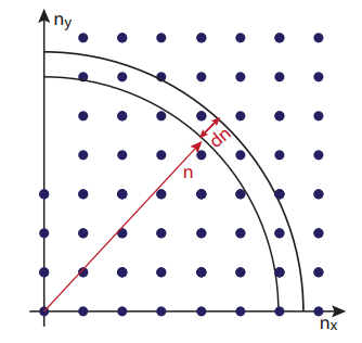
As for the 1D case, we have a quantization of the momentum (and hence of the wave-number \(k\)) in order to fit the wavefunction in the box. Here we just have a quantization in all 3 directions:
\[k_{x}=\frac{2 \pi}{L} n_{x}, \quad k_{y}=\frac{2 \pi}{L} n_{y}, \quad k_{z}=\frac{2 \pi}{L} n_{z} \nonumber\]
(with \(n\) integers). Then, going to spherical coordinates, we can count the number of states in a spherical shell between \(n\) and \(n + dn\) to be \(d N_{s}=4 \pi n^{2} d n\). Expressing this in terms of \(k\), we have \(d N_{s}=4 \pi k^{2} d k \frac{L^{3}}{(2 \pi)^{3}}\). If we consider just a small solid angle \(d \Omega\) instead of \(4 \pi\) we have then the number of state \(d N_{s}=\frac{L^{3}}{(2 \pi)^{3}} k^{2} d k d \Omega\). Since \(E=\hbar k c=\hbar \omega\), we finally obtain the density of states:
\[\rho(E)=\frac{d N_{s}}{d E}=\frac{L^{3}}{(2 \pi)^{3}} k^{2} \frac{d k}{d E} d \Omega=\frac{L^{3}}{(2 \pi)^{3}} \frac{k^{2}}{\hbar c} d \Omega=\frac{\omega^{2}}{\hbar c^{3}} \frac{L^{3}}{(2 \pi)^{3}} d \Omega \nonumber\]
The vector potential
Next we consider the potential causing the transition. The interaction of a particle with the e.m. field can be expressed in terms of the vector potential \( \hat{\vec{A}}\) of the e.m. field as:
\[\hat{V}=\frac{e}{m c} \hat{\vec{A}} \cdot \hat{\vec{p}} \nonumber\]
where \( \hat{\vec{p}}\) is the particle’s momentum. The vector potential \( \hat{\vec{A}}\) in QM is an operator that can create or annihilate photons,
\[\hat{\vec{A}}=\sum_{k} \sqrt{\frac{2 \pi \hbar c^{2}}{V \omega_{k}}}\left(\hat{a}_{k} e^{i \vec{k} \cdot \vec{r}}+\hat{a}_{k}^{\dagger} e^{-i \vec{k} \cdot \vec{r}}\right) \vec{\epsilon}_{k} \nonumber\]
where \( \hat{a}_{k}\left(\hat{a}_{k}^{\dagger}\right)\) annihilates (creates) one photon of momentum \( \vec{k}\). Also, \(\vec{\epsilon}_{k} \) is the polarization of the e.m. field. Since gamma decay (and many other atomic and nuclear processes) is able to create photons (or absorb them) it makes sense that the operator describing the e.m. field would be able to describe the creation and annihilation of photons. The second characteristic of this operator are the terms \(\propto e^{-i \vec{k} \cdot \vec{r}} \) which describe a plane wave, as expected for e.m. waves, with momentum \(\hbar k \) and frequency \(ck\).
Dipole transition for gamma decay
To calculate the transition rate from the Fermi’s Golden rule,
\[W=\frac{2 \pi}{\hbar}\left|\left\langle\psi_{f}|\hat{V}| \psi_{i}\right\rangle\right|^{2} \rho\left(E_{f}\right), \nonumber\]
we are really only interested in the matrix element \( \left\langle\psi_{f}|\hat{V}| \psi_{i}\right\rangle\), where the initial state does not have any photon, and the final has one photon of momentum \(\hbar k \) and energy \( \hbar \omega=\hbar k c .\). Then, the only element in the sum above for the vector potential that gives a non-zero contribution will be the term \( \propto \hat{a}_{k}^{\dagger}\), with the appropriate \(\vec{k} \) momentum:
\[V_{i f}=\frac{e}{m c} \sqrt{\frac{2 \pi \hbar c^{2}}{V \omega_{k}}} \vec{\epsilon}_{k} \cdot\left\langle\hat{\vec{p}} e^{-i \vec{k} \cdot \vec{r}}\right\rangle \nonumber\]
This can be simplified as follow. Remember that \( \left[\hat{\vec{p}}^{2}, \hat{\vec{r}}\right]=-2 i \hbar \hat{\vec{p}}\). Thus we can write, \( \hat{\vec{p}}=\frac{i}{2 \hbar}\left[\hat{\vec p}^{2}, \hat{\vec{r}}\right]=\frac{i m}{\hbar}\left[\frac{\hat{\vec p}^{2}}{2 m}, \hat{\vec{r}}\right]= \frac{i m}{\hbar}\left[\frac{\hat{\vec p}^{2}}{2 m}+V_{n u c}(\hat{\vec{r}}), \hat{\vec{r}}\right]\). We introduced the nuclear Hamiltonian \(\mathcal{H}_{n u c}=\frac{\hat{\vec p}^{2}}{2 m}+V_{n u c}(\hat{\vec{r}}) \): thus we have \( \hat{\vec{p}}=\frac{i m}{\hbar}\left[\mathcal{H}_{n u c}, \hat{\vec{r}}\right]\). Taking the expectation value
\[\left\langle\psi_{f}|\hat{\vec{p}}| \psi_{i}\right\rangle=\frac{i m}{\hbar}\left(\left\langle\psi_{f}\left|\mathcal{H}_{n u c} \hat{\vec{r}}\right| \psi_{i}\right\rangle-\left\langle\psi_{f}\left|\hat{\vec{r}} \mathcal{H}_{n u c}\right| \psi_{i}\right\rangle\right) \nonumber\]
and remembering that \(\left|\psi_{i, f}\right\rangle\) are eigenstates of the Hamiltonian, we have
\[\left\langle\psi_{f}|\hat{\vec{p}}| \psi_{i}\right\rangle=\frac{i m}{\hbar}\left(E_{f}-E_{i}\right)\left\langle\psi_{f}|\hat{\vec{r}}| \psi_{i}\right\rangle=i m \omega_{k}\left\langle\psi_{f}|\hat{\vec{r}}| \psi_{i}\right\rangle, \nonumber\]
where we used the fact that \( \left(E_{f}-E_{i}\right)=\hbar \omega_{k}\) by conservation of energy. Thus we obtain
\[V_{i f}=\frac{e}{m c} \sqrt{\frac{2 \pi \hbar c^{2}}{V \omega_{k}}} i m \omega \vec{\epsilon}_{k} \cdot\left\langle\hat{\vec{r}} e^{-i \vec{k} \cdot \vec{r}}\right\rangle=i \sqrt{\frac{2 \pi \hbar e^{2} \omega_{k}}{V}} \vec{\epsilon}_{k} \cdot\left\langle\hat{\vec{r}} e^{-i \vec{k} \cdot \vec{r}}\right\rangle \nonumber\]
We have seen that the wavelengths of gamma photons are much larger than the nuclear size. Then \( \vec{k} \cdot \vec{r} \ll 1\) and we can make an expansion in series : \(e^{-\vec{k} \cdot \vec{r}} \sim \sum_{l} \frac{1}{l !}(-i \vec{k} \cdot \vec{r})^{l}=\sum_{l} \frac{1}{l !}(-i k r \cos \vartheta)^{l}\). This series is very similar in meaning to the multipole series we saw for the classical case.
For example, for \(l\) = 0 we obtain:
\[V_{i f}=\sqrt{\frac{2 \pi \hbar e^{2} \omega_{k}}{V}}\langle\hat{\vec{r}}\rangle \cdot \vec{\epsilon}_{k} \nonumber\]
which is the dipolar approximation, since it can be written also using the electric dipole operator \(e \hat{\vec{r}} \).
The angle between the polarization of the e.m. field and the position \( \hat{\vec{r}}\) is \(\langle\hat{\vec{r}}\rangle \cdot \vec{\epsilon}=\langle\hat{\vec{r}}\rangle \sin \vartheta\)
The transition rate for the dipole radiation, \(W \equiv \lambda(E 1)\) is then:
\[\lambda(E 1)=\frac{2 \pi}{\hbar}\left|\left\langle\psi_{f}|\hat{V}| \psi_{i}\right\rangle\right|^{2} \rho\left(E_{f}\right)=\frac{\omega^{3}}{2 \pi c^{3} \hbar}|\langle\hat{\vec{r}}\rangle|^{2} \sin ^{2} \vartheta d \Omega \nonumber\]
and integrating over all possible direction of emission (\(\int_{0}^{2 \pi} d \varphi \int_{0}^{\pi}\left(\sin ^{2} \vartheta\right) \sin \vartheta d \vartheta=2 \pi \frac{4}{3}\)):
\[\lambda(E 1)=\frac{4}{3} \frac{e^{2} \omega^{3}}{\hbar c^{3}}|\langle\hat{\vec{r}}\rangle|^{2} \nonumber\]
Multiplying the transition rate (or photons emitted per unit time) by the energy of the photons emitted we obtain the radiated power, \(P=W \hbar \omega\):
\[P=\frac{4}{3} \frac{e^{2} \omega^{4}}{c^{3}}|\langle\hat{\vec{r}}\rangle|^{2} \nonumber\]
Notice the similarity of this formula with the classical case:
\[P_{E 1}=\frac{1}{3} \frac{e^{2} \omega^{4}}{c^{3}}\left|\vec{r}_{0}\right|^{2} \nonumber\]
We can estimate the transition rate by using a typical energy \( E=\hbar \omega\) for the photon emitted (equal to a typical energy difference between excited and ground state nuclear levels) and the expectation value for the dipole (\( |\langle\hat{\vec{r}}\rangle| \sim R_{n u c} \approx r_{0} A^{1 / 3}\)). Then, the transition rate is evaluated to be
\[\lambda(E 1)=\frac{e^{2}}{\hbar c} \frac{E^{3}}{(\hbar c)^{3}} r_{0}^{2} A^{2 / 3}=1.0 \times 10^{14} A^{2 / 3} E^{3} \nonumber\]
(with E in MeV). For example, for A = 64 and E = 1MeV the rate is \(\lambda \approx 1.6 \times 10^{15} s^{-1} \) or \( \tau=10^{-15}\) (femtoseconds!) for E = 0.1MeV \( \tau\) is on the order of picoseconds.
Because of the large energies involved, very fast processes are expected in the nuclear decay from excited states, in accordance with Fermi’s Golden rule and the energy/time uncertainty relation.
Extension to Multipoles
We obtained above the transition rate for the electric dipole, i.e. when the interaction between the nucleus and the e.m. field is described by an electric dipole and the emitted radiation has the character of electric dipole radiation. This type of radiation can only carry out of the nucleus one quantum of angular momentum (i.e. \(\Delta l=\pm 1 \), between excited and ground state). In general, excited levels differ by more than 1 \(l\), thus the radiation emitted need to be a higher multipole radiation in order to conserve angular momentum.
Electric Multipoles
We can go back to the expansion of the radiation interaction in multipoles:
\[\hat{V} \sim \sum_{l} \frac{1}{l !}(i \hat{\vec{k}} \cdot \hat{\vec{r}})^{l} \nonumber\]
Then the transition rate becomes:
\[\lambda(E l)=\frac{8 \pi(l+1)}{l[(2 l+1) ! !]^{2}} \frac{e^{2}}{\hbar c}\left(\frac{E}{\hbar c}\right)^{2 l+1}\left(\frac{3}{l+3}\right)^{2} c\langle|\hat{\vec{r}}|\rangle^{2 l} \nonumber\]
Notice the strong dependence on the \(l\) quantum number. Setting again \(|\langle\hat{\vec{r}}\rangle| \sim r_{0} A^{1 / 3}\) we also have a strong dependence on the mass number.
Thus, we have the following estimates for the rates of different electric multipoles:
- \(\lambda(E 1)=1.0 \times 10^{14} A^{2 / 3} E^{3}\)
- \(\lambda(E 2)=7.3 \times 10^{7} A^{4 / 3} E^{5}\)
- \(\lambda(E 3)=34 A^{2} E^{7}\)
- \(\lambda(E 4)=1.1 \times 10^{-5} A^{8 / 3} E^{9}\)
Magnetic Multipoles
The e.m. potential can also contain magnetic interactions, leading to magnetic transitions. The transition rates can be calculated from a similar formula:
\[\lambda(M l)=\frac{8 \pi(l+1)}{l[(2 l+1) ! !]^{2}} \frac{e^{2}}{\hbar c} \frac{E^{2 l+1}}{\hbar c}\left(\frac{3}{l+3}\right)^{2} c\langle|\hat{\vec{r}}|\rangle^{2 l-2}\left[\frac{\hbar}{m_{p} c}\left(\mu_{p}-\frac{1}{l+1}\right)\right] \nonumber\]
where \(\mu_{p} \) is the magnetic moment of the proton (and \( m_{p}\) its mass).
Estimates for the transition rates can be found by setting \(\mu_{p}-\frac{1}{l+1} \approx 10\):
- \(\lambda(M 1)=5.6 \times 10^{13} E^{3}\)
- \(\lambda(M 2)=3.5 \times 10^{7} A^{2 / 3} E^{5}\)
- \(\lambda(M 3)=16 A^{4 / 3} E^{7}\)
- \(\lambda(M 4)=4.5 \times 10^{-6} A^{2} E^{9}\)
Selection Rules
The angular momentum must be conserved during the decay. Thus the difference in angular momentum between the initial (excited) state and the final state is carried away by the photon emitted. Another conserved quantity is the total parity of the system.
Parity change
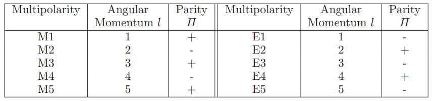
The parity of the gamma photon is determined by its character, either magnetic or electric multipole. We have
\[\Pi_{\gamma}(E l)=(-1)^{l} \quad \text { Electric multipole } \nonumber\]
\[\Pi_{\gamma}(M l)=(-1)^{l-1} \quad \text { Magnetic multipole } \nonumber\]
Then if we have a parity change from the initial to the final state \(\Pi_{i} \rightarrow \Pi_{f}\) this is accounted for by the emitted photon as:
\[\Pi_{\gamma}=\Pi_{i} \Pi_{f} \nonumber\]
This of course limits the type of multipole transitions that are allowed given an initial and final state.
\[\Delta \Pi=\mathrm{no} \rightarrow \text { Even Electric, Odd Magnetic } \nonumber\]
\[\Delta \Pi=\text { yes } \rightarrow \text { Odd Electric, Even Magnetic } \nonumber\]
Angular momentum
From the conservation of the angular momentum:
\[\hat{\vec{I}}_{i}=\hat{\vec{I}}_{f}+\hat{\vec{L}}_{\gamma} \nonumber\]
the allowed values for the angular momentum quantum number of the photon, \(l\), are restricted to
\[l_{\gamma}=\left|I_{i}-I_{f}\right|, \ldots, I_{i}+I_{f} \nonumber\]
Once the allowed \(l\) have been found from the above relationship, the character (magnetic or electric) of the multipole is found by looking at the parity.
In general then, the most important transition will be the one with the lowest allowed \(l\), \( \Pi\). Higher multipoles are also possible, but they are going to lead to much slower processes.
Dominant Decay Modes
In general we have the following predictions of which transitions will happen:
- The lowest permitted multipole dominates
- Electric multipoles are more probable than the same magnetic multipole by a factor ∼ 102 (however, which one is going to happen depends on the parity)
\[\frac{\lambda(E l)}{\lambda(M l)} \approx 10^{2} \nonumber\] - Emission from the multipole \(l\) + 1 is 10−5 times less probable than the \(l\)-multipole emission.
\[\frac{\lambda(E, l+1)}{\lambda(E l)} \approx 10^{-5}, \quad \frac{\lambda(M, l+1)}{\lambda(M l)} \approx 10^{-5} \nonumber\] - Combining 2 and 3, we have:
\[\frac{\lambda(E, l+1)}{\lambda(M l)} \approx 10^{-3}, \quad \frac{\lambda(M, l+1)}{\lambda(E l)} \approx 10^{-7} \nonumber\]
Thus E2 competes with M1 while that’s not the case for M2 vs. E1
Internal conversion
What happen if no allowed transitions can be found? This is the case for even-even nuclides, where the decay from the 0+ excited state must happen without a change in angular momentum. However, the photon always carries some angular momentum, thus gamma emission is impossible.
Then another process happens, called internal conversion:
\[\stackrel{A}{Z} X^{*} \rightarrow_{Z}^{A} X+e^{-} \nonumber\]
where \({}^A_Z X \) is a ionized state and \(e^{-} \) is one of the atomic electrons.
Besides the case of even-even nuclei, internal conversion is in general a competing process of gamma decay (see Krane for more details).