
3.1: Cornu's Spiral


- Last updated
- Jun 21, 2021
- Save as PDF

( \newcommand{\kernel}{\mathrm{null}\,}\)
If a parallel beam of light from a distant source encounters an obstacle, the shadow of the obstacle is not a simple geometric shadow but is, rather, a diffraction pattern. For example, it is well known that the diffraction pattern formed by a slit looks like the function shown in Figure 1.
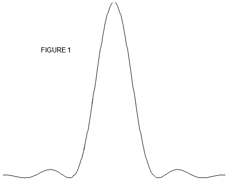
Such diffraction is called Fraunhofer diffraction.
If, however, the source of light is not distant, but is close to the diffracting obstacle so that the incident waves are not plane waves, the diffraction pattern will look somewhat different. Such diffraction is called Fresnel diffraction, and its theory is, unsurprisingly, a little more difficult than the theory for Fraunhofer diffraction.
If the source of light is a point source, so that the incident wavefronts are spherical, the detailed quantitative theory is not at all easy. If the incident wavefronts, however, are cylindrical (say from a linear source) the analysis, which is two dimensional, is a little more tractable. Cornu’s spiral is a graphical device that enables us to compute and predict the Fresnel diffraction pattern from various simple obstacles.
“Cornu”, by the way, is French for “horned”, and can also mean “spiral” - i.e. like the horns of a bighorn sheep or of an ibex. Because of this I wondered, when I first heard about Cornu’s spiral, whether it should really be called a “cornu spiral”, rather than Cornu’s spiral. However, it is correctly named Cornu’s spiral after a real nineteenth century French scientist, Marie Alfred Cornu. The mathematical properties of the spiral had been examined by various mathematicians (for example, Euler) before Cornu, but it has acquired the name of Cornu because of its application by Cornu to the theory of Fresnel diffraction.
Let us look, in Figure III.2, at the geometry of a cylindrical wavefront from a linear source at O.
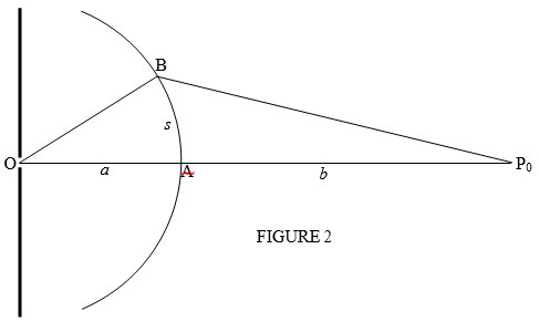
Introduce a dimensionless variable v by
v=√2(a+b)abλ s.
where λ is the wavelength of the light.
Theory shows that the intensity (square of the amplitude) of the radiation received at the point P0 from the portion AB of arc-length s of the wavefront is proportional to
(∫v0cos12πu2du)2 + (∫v0sin12πu2du)2.
Here
C = ∫v0cos12πu2duandS = ∫v0sin12πu2du
are the Fresnel integrals.
The derivation of Equation (3) may be somewhat heavy-going, and we shall relegate it to Appendix A at the end of this chapter. For the time being, we shall accept Equation (3) as being correct, and we shall see how to use it to construct the Cornu spiral and how the spiral can be used to compute the forms of the shadows produced by various obstacles. In Equations (4), u is just a dummy variable. C and S are functions of v, which is proportional to s. They must be integrated numerically, and I have provided a brief table of them in Appendix B.
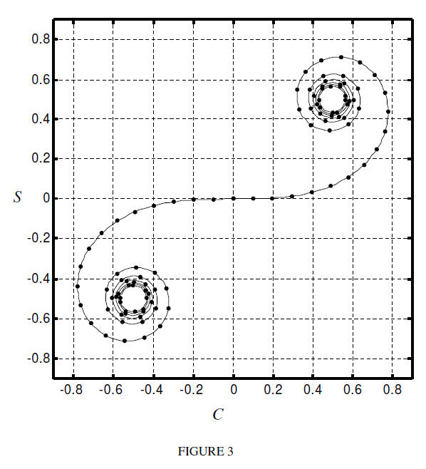
The Cornu spiral is a graph of S versus C. Figure III.3 shows such a graph. Better ones exist in the literature, but this one will suffice to show how it is used. However, I shall shortly suggest that, while it is fun to use the spiral, for precise work it is preferable to compute the forms of the shadows numerically rather than graphically. The spiral was useful in the days before high-speed computers, but today one can compute the Fresnel integrals instantaneously, and hence we can compute the forms of the shadow, using the spiral perhaps to guide us. A word of warning, though. The rapid and accurate computation of the Fresnel integrals requires some care in programming, for the integrand changes rapidly with the variable u. In preparing the graphs and tables in this note, I found that Simpson’s Rule was inadequate - it worked provided I used a large number of intervals, but this slowed down the computation. I was able to get better and faster results with Gaussian quadrature.
The dimensionless variable v (which is proportional to s - see Equation 1) is measured along the spiral. I have drawn dots on the spiral for every 0.1 increment in v. I haven’t labelled the numerical values of v beside the dots, but feel free to do so if you wish. Note that, as v→±∞, C and S→±12. The intensity at P is proportional to the square of the distance between these two limiting points (12,12) and (−12,−12). The distance between these points is √2, and the square of the distance is 2. Thus, with no obstacle between the source and the point P, the amplitude of the radiation at P is √2 (arbitrary units), and the intensity at P is 2 (arbitrary units).
In what follows, we are going to put three obstacles in front of the light source and we are going to compute the Fresnel diffraction pattern (i.e. the structure of the shadow.) The three obstacles will be a single straight edge, a slit between two straight edges, and an opaque strip:
All the time recall that the distance s along the wavefront is linearly related to the distance v along the Cornu spiral.
We’ll start with the single straight edge.
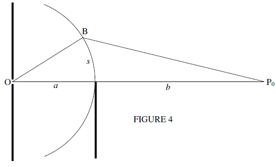
At the point P0 we see all of the upper part of the wavefront. That is, we see along the Cornu spiral from v=0 to where the spiral converges at C = 12, S = 12. The amplitude of the radiation at P is proportional to the distance between these two points, which is 1√2, and the intensity at P is proportional to the square of this, which is 12, which is one quarter of the intensity when the light was unobstructed by any obstacle.
Now let us see what the intensity is at a point P some way above the axis (Figure 5).
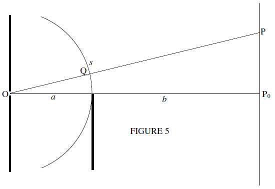
The distance s is must now be measured not from the edge of the obstacle, but from the point Q. At P we see more of the wavefront than we did at P0. We see all of s above Q, as well as some negative values of s below Q. The amplitude at P, then, corresponds to the length of the chord in Figure III.6, in which the negative v is related to the negative s by Equation (1). We see that, as we move P upwards in Figure 5, We take in more and more negative s, and more and more negative v in the Cornu spiral.
.PNG?revision=1&size=bestfit&width=503&height=563)
Thus, as P moves upwards in Figure 5, we keep the upper end of the chord in Figure 6 fixed and we move the lower end around the spiral. The length of the chord is proportional to the amplitude of the light received at P, and its square is proportional to its intensity.
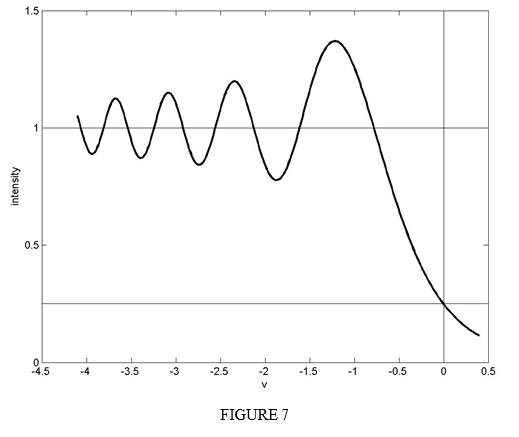
We can use a ruler and the spiral to determine the intensity as a function of v and hence of s, and this would have been an appropriate procedure before the advent of high-speed computers. To delineate the intensity as a function of v by computer, as we move along the spiral, for each value of v we calculate C and S and then calculate the intensity from the square of the length of the chord, which is
(12−C)2 + (12−S)2.
This is what I did for Figure 7 except that I divided this expression by two, so that an intensity of one represents the intensity at P0 in the absence of any obstacle. A reader who tries to duplicate this will soon appreciate the value of programming a fast and accurate method of evaluating the Fresnel integrals.
The portion to the right of v = 0 is within the geometric shadow.
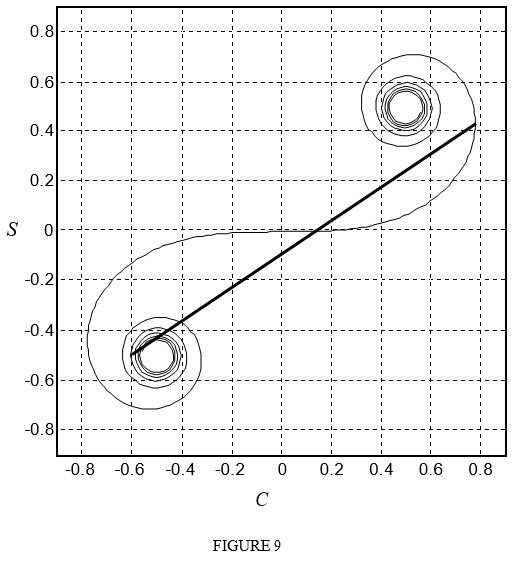
Now we’ll look at what happens when the obstacle is a slit between two straight edges. We’ll suppose that the width of the slit is Δs, corresponding to a distance along the spiral Δv = √2(a+b)abλ Δs. In the calculations that I have done below, I have taken Δv to be 4.0. The point P (see Figure 8) is receiving energy from the part of the wavefront between s − Δs and s, corresponding to a chord on the spiral spanning a distance Δv along the spiral. As the point P moves upward along the screen, so the chord slides along the spiral (see Figure 9), keeping Δv constant
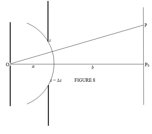
For each position of the chord, we need to calculate the Fresnel integrals Cu, Su of the upper end of the chord and the Fresnel integrals Cl,Sl of the lower end of the chord and then calculate the square of the length of the chord (and then divide by two, so that an intensity of 1 is the intensity when the light is unobstructed). That is, we calculate
12[(Cu−Cl)2 + (Su −S1)2]
I got the result shown in Figure 10, using a slit width corresponding to Δv= 4.
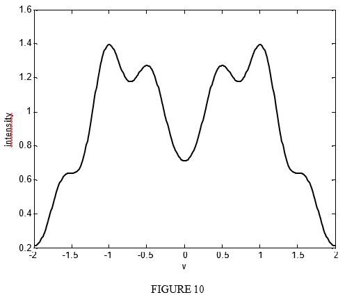
The positions v= ±2 correspond to the edge of he geometric shadow. The intensity has not fallen to zero there - some light spills over into the geometric shadow.
The details of the diffraction pattern are very sensitive to the value of Δv. That is to say to Δs. That is to say to the slit width. Figure 11, for example, shows the same calculation but for Δv = 3.9 rather than 0.4.
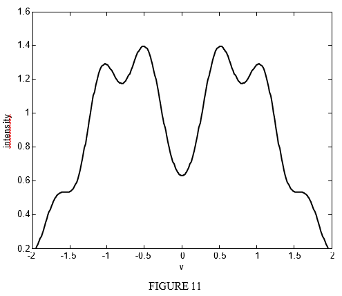
As the slit width is changed, sometimes there will be a dip at v = 0, and sometimes a maximum. Generally, a large Δv results in a more complicated pattern, and a smaller Δv results in a simpler pattern. As Δv becomes smaller, the pattern approaches the familiar Fraunhofer diffraction pattern for a slit, as in Figure 1.
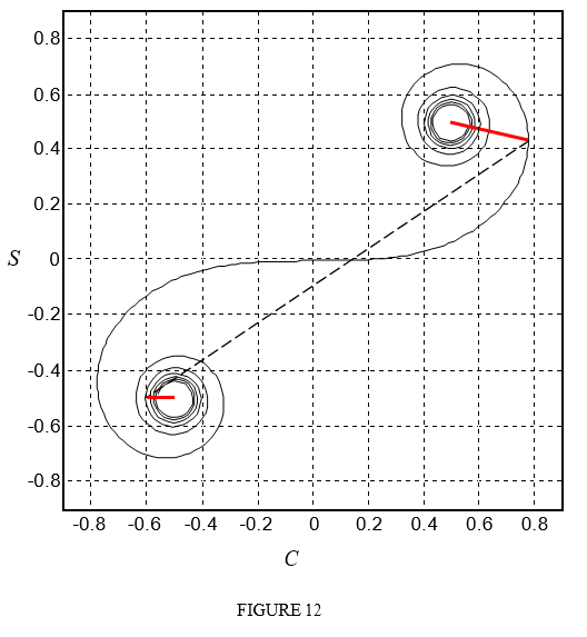
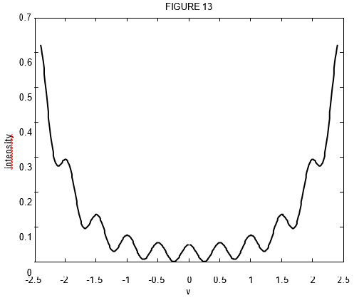
Now let us choose as the obstacle a single opaque strip. I’ll make the width of the strip equal to the width of the slit in the example of Figure 10, which corresponds to a distance along the spiral of Δv = 4. Instead of sliding the chord of Figure III.10 along the spiral, we have to slide the two complementary chords shown in Figure 12. We have to calculate the same Fresnel integrals Cu, Su, Cl, Sl as before, but this time the resultant of the two, added as vectors, and normalized so that the unobstructed intensity is 1, is 12[(1−Cu+Cl)2 + (1−Su +S1)2]. I obtain the result shown in Figure 13.
The key to doing these calculations successfully is to have an efficient, fast and accurate routine for calculating the Fresnel integrals. In each of these graphs each of the Fresnel integrals (sine and cosine) was calculated by numerical integration about 400 times. I found Simpson’s Rule was inadequate, so I used Gaussian Quadrature.
APPENDIX A
In the above notes, I have described what the Fresnel integrals and the Cornu spiral are, and how to use them in some simple cases. I have not shown why it is that the diffraction patterns can be generated by the Fresnel integrals, or how to derive Equation (3). I hope sometime to derive this and explain the rationale behind the theory in this Appendix at some later date. I’m afraid I can’t say when I expect to get round to doing this. Could be this year, next year, sometime, never...
APPENDIX B
| v | C | S |
|---|---|---|
| 0.10 | 0.1000 | 0.0005 |
| 0.20 | 0.1999 | 0.0042 |
| 0.30 | 0.2994 | 0.0141 |
| 0.40 | 0.3975 | 0.0334 |
| 0.50 | 0.4923 | 0.0647 |
| 0.60 | 0.5811 | 0.1105 |
| 0.70 | 0.6597 | 0.1721 |
| 0.80 | 0.7228 | 0.2493 |
| 0.90 | 0.7648 | 0.3398 |
| 1.00 | 0.7799 | 0.4383 |
| 1.10 | 0.7638 | 0.5365 |
| 1.20 | 0.7154 | 0.6234 |
| 1.30 | 0.6385 | 0.6863 |
| 1.40 | 0.5431 | 0.7135 |
| 1.50 | 0.4453 | 0.6975 |
| 1.60 | 0.3655 | 0.6389 |
| 1.70 | 0.3238 | 0.5492 |
| 1.80 | 0.3336 | 0.4509 |
| 1.90 | 0.3945 | 0.3733 |
| 2.00 | 0.4883 | 0.3434 |
| 2.10 | 0.5816 | 0.3743 |
| 2.20 | 0.6363 | 0.4557 |
| 2.30 | 0.6266 | 0.5532 |
| 2.40 | 0.5550 | 0.6197 |
| 2.50 | 0.4574 | 0.6192 |
| 2.60 | 0.3889 | 0.5500 |
| 2.70 | 0.3925 | 0.4529 |
| 2.80 | 0.4675 | 0.3915 |
| 2.90 | 0.5624 | 0.4101 |
| 3.00 | 0.6057 | 0.4963 |
| 3.10 | 0.5616 | 0.5818 |
| 3.20 | 0.4663 | 0.5933 |
| 3.30 | 0.4057 | 0.5193 |
| 3.40 | 0.4385 | 0.4296 |
| 3.50 | 0.5326 | 0.4152 |
| 3.60 | 0.5879 | 0.4923 |
| 3.70 | 0.5419 | 0.5750 |
| 3.80 | 0.4481 | 0.5656 |
| 3.90 | 0.4223 | 0.4752 |
| 4.00 | 0.4984 | 0.4205 |
| 4.10 | 0.5737 | 0.4758 |
| 4.20 | 0.5417 | 0.5632 |
| 4.30 | 0.4494 | 0.5540 |
| 4.40 | 0.4383 | 0.4623 |
| 4.50 | 0.5260 | 0.4343 |
| 4.60 | 0.5672 | 0.5162 |
| 4.70 | 0.4914 | 0.5671 |
| 4.80 | 0.4338 | 0.4967 |
| 4.90 | 0.5002 | 0.4351 |
| 5.00 | 0.5636 | 0.4992 |
| 5.10 | 0.4998 | 0.5624 |